↗ OpenReview ↗ NeurIPS Homepage ↗ Chat
TL;DR#
Vision Transformers (ViTs) are powerful but demand significant computational resources, hindering their deployment on resource-constrained devices. Existing approaches train multiple ViT models of different sizes to accommodate varying hardware capabilities; however, this necessitates training and storing each model separately, resulting in inefficiency and scalability limitations. This necessitates the development of flexible and adaptable ViT architectures.
HydraViT addresses this by employing stochastic training to induce multiple subnetworks within a single ViT model. By dynamically selecting subsets of attention heads and embedding dimensions during inference, HydraViT achieves scalability across various hardware constraints without sacrificing performance. Experimental results demonstrate that HydraViT achieves better accuracy than existing methods with similar GMACs and throughput. This flexible approach resolves the scalability issue, making ViTs more adaptable to resource-limited scenarios.
Key Takeaways#
Why does it matter?#
This paper is important because it introduces a novel approach to building scalable Vision Transformers (ViTs), addressing the limitations of existing methods that rely on training and storing multiple models of varying sizes. HydraViT offers a significant advancement by achieving scalability through stochastic training, enabling adaptability across diverse hardware constraints while maintaining performance. This opens new avenues for research into efficient and adaptable ViT architectures for various resource-constrained applications.
Visual Insights#
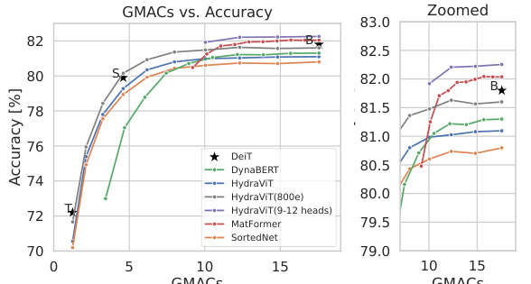
This figure compares the performance of HydraViT against several baseline models (DeiT, DynaBERT, MatFormer, and SortedNet) on the ImageNet-1K dataset. Two performance metrics are shown: GMACs (giga multiply-accumulate operations) representing computational complexity and throughput (images/second) representing inference speed. The plots reveal that HydraViT achieves superior accuracy compared to the baselines for similar levels of computational cost or speed, especially when trained with a wider range of heads (9-12). The figure highlights HydraViT’s scalability and efficiency.

This table shows the configurations of three different sizes of Vision Transformers (ViTs): ViT-Ti, ViT-S, and ViT-B. It lists the number of layers, the embedding dimension (‘Dim’), the number of attention heads, the dimension of each head, and the total number of parameters in each model. The table highlights the key differences in architecture and model size among these ViT variations.
In-depth insights#
Scalable ViT Design#
Designing scalable Vision Transformers (ViTs) is crucial for deploying them on devices with varying resource constraints. A key challenge lies in the Multi-Head Attention (MHA) mechanism’s inherent computational demands. Simply training multiple ViT models of different sizes is inefficient. Innovative approaches are needed to create a single model that adapts to different hardware capabilities. Dynamically adjusting the number of attention heads and embedding dimensions during both training and inference offers a promising solution. This allows the model to gracefully scale its complexity based on available resources, maximizing performance across diverse hardware. Stochastic training techniques can further enhance efficiency by jointly training multiple subnetworks within a single architecture. This approach necessitates careful consideration of how to maintain accuracy while allowing the model to operate with reduced computational resources. Careful evaluation across various hardware platforms is critical to assess the true scalability and efficiency gains of the design. The potential trade-offs between accuracy and resource utilization must be thoroughly examined. Such an approach ultimately aims to make the powerful capabilities of ViTs accessible on a much wider range of devices.
Stochastic Training#
The concept of ‘Stochastic Training’ in the context of a vision transformer model, like the one presented, is crucial for achieving scalability. The core idea involves using a random sampling process to select subnetworks within the model during the training phase. This approach avoids the computational burden of training all possible subnetworks independently, significantly reducing the training time and resource consumption. By randomly selecting subsets of attention heads and embedding dimensions, the model implicitly learns to adapt to various resource constraints. This stochastic approach effectively orders the attention heads and corresponding embedding vectors based on their learned importance. The model learns to extract relevant features with fewer heads and smaller dimensions when needed, allowing for seamless adaptation during inference to different hardware capabilities. The effectiveness is demonstrated through the ability to achieve similar accuracy to that of multiple separately-trained models, but with significantly less training effort. However, it is important to note the limitations in training, such as the increased computational demand during stochastic training, and the trade-off between the number of epochs and the accuracy of the smaller subnetworks.
Subnetwork Sampling#
Subnetwork sampling is a crucial technique within the HydraViT architecture, significantly impacting its efficiency and accuracy. The core idea is to stochastically select a subset of the network’s attention heads and their corresponding embedding dimensions during training. This approach allows for the efficient training of a single model capable of producing multiple subnetworks with varying resource demands. The choice of sampling distribution (uniform or weighted) influences the training process. A uniform distribution offers simplicity and ensures all subnetworks receive attention, leading to good generalization. Conversely, a weighted distribution allows for prioritizing specific subnetworks, potentially improving accuracy on resource-constrained devices at the cost of slightly reduced performance on others. This method creates flexibility and scalability by enabling HydraViT to adapt to different hardware resources during inference by dynamically selecting a subnetwork based on the available resources. The experimental results highlight the effectiveness of this approach for achieving scalability without compromising accuracy to a large extent. The choice between uniform and weighted sampling presents a trade-off between generalization and targeted optimization, allowing users to tailor the model to their specific deployment scenario.
Performance Analysis#
A thorough performance analysis of any Vision Transformer (ViT) model should encompass several key aspects. Accuracy is paramount, comparing the model’s performance against established baselines on standard datasets like ImageNet. Computational efficiency, measured by GMACs (giga multiply-accumulate operations), is critical, especially for resource-constrained deployments. Throughput (images processed per second) directly impacts real-world usability, and this should be evaluated on various hardware platforms to highlight scalability. Memory requirements (RAM) also play a significant role, impacting deployment feasibility on different devices. Finally, a robust analysis should investigate the model’s performance on diverse datasets, including variations of ImageNet or other challenging benchmarks, to showcase its generalization capabilities and robustness. Comparing performance across different subsets of the model is vital for understanding scalability, demonstrating the trade-offs between accuracy and resource usage. The results should be presented clearly, using graphs and tables to effectively visualize the trade-offs, making it easy to interpret the model’s strengths and weaknesses in various deployment scenarios.
Future Work#
Future research directions stemming from this HydraViT paper could explore several promising avenues. Extending HydraViT’s adaptability to even more diverse hardware is crucial, potentially encompassing a wider range of mobile devices and embedded systems beyond those initially tested. A significant enhancement would involve developing more sophisticated subnetwork selection strategies, moving beyond uniform random sampling to incorporate techniques like reinforcement learning or Bayesian optimization for more efficient resource allocation at inference time. Investigating the impact of different training schedules and optimization algorithms on the performance and efficiency of HydraViT is warranted. Furthermore, a comprehensive analysis of the model’s robustness to various forms of adversarial attacks and noise would solidify its practical viability. Finally, exploring the potential of HydraViT as a foundational architecture for other vision tasks beyond image classification (e.g., object detection, segmentation) could open up new frontiers in efficient and adaptive computer vision systems.
More visual insights#
More on figures
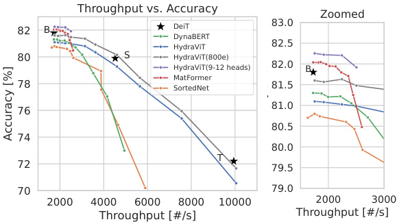
This figure compares the performance of HydraViT against several baseline models (DeiT, DynaBERT, MatFormer, and SortedNet) on the ImageNet-1K dataset. The comparison is shown across two key metrics: GMACs (giga multiply-accumulate operations) and throughput (images processed per second). It demonstrates that HydraViT achieves superior performance (accuracy) compared to the baselines, especially when trained with 9-12 heads and for longer epochs, showcasing its scalability and efficiency.

This figure illustrates the architecture of HydraViT, highlighting the key components: Patch Embedding, Norm, Multi-Head Attention, Norm, and MLP layers. The figure emphasizes the selection of subnetworks within the architecture, indicated by the dotted lines and the ‘Subnetwork Selection’ label on the right side. This highlights HydraViT’s capacity to dynamically choose subnetworks based on available hardware resources.

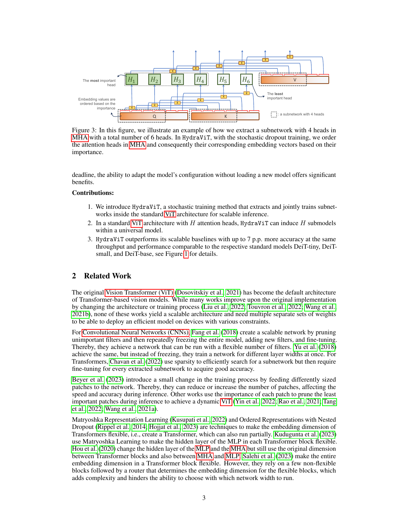
This figure illustrates how HydraViT extracts subnetworks. It shows a multi-head attention (MHA) layer with six heads (H1-H6). During stochastic dropout training, the heads are ordered by importance. The figure highlights how a subnetwork is created by selecting the top k most important heads and their corresponding embedding vectors. In this example, a subnetwork with four heads is shown. The importance ordering of heads allows HydraViT to dynamically select the appropriate subnetwork at inference time based on available hardware resources.

This figure illustrates how HydraViT extracts subnetworks from the MLP and NORM layers. It shows how HydraViT selects portions of activation maps and weight matrices based on the number of heads used, effectively creating subnetworks of varying sizes. The figure uses the examples of 3, 6, and 12 heads (corresponding to ViT-Ti, ViT-S, and ViT-B) for simplicity and clarity.

This figure compares the performance of HydraViT against several baselines (DeiT, DynaBERT, MatFormer, SortedNet) on the ImageNet-1K dataset. Two plots are shown: one illustrating the relationship between GMACs (giga multiply-accumulate operations) and accuracy, and the other showing the relationship between throughput and accuracy. HydraViT demonstrates improved accuracy compared to the baselines at similar GMACs and throughput levels, especially when trained with 9-12 heads, showcasing its scalability and efficiency.
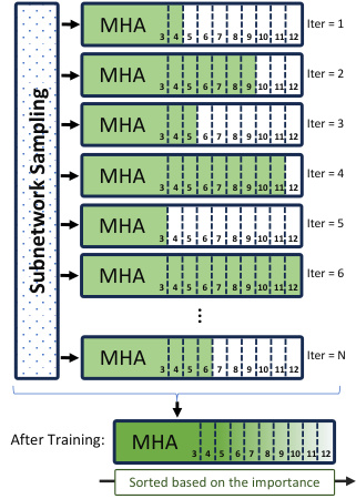
This figure illustrates the stochastic dropout training process in HydraViT. In each iteration, a subset of attention heads (a subnetwork) is randomly selected using a uniform distribution. The selected heads and their corresponding embedding vectors are involved in the backpropagation and forward paths. After training, this process results in an ordering of the attention heads based on their importance. The most important heads are used first, facilitating flexible and efficient inference using only the most relevant parts of the network.

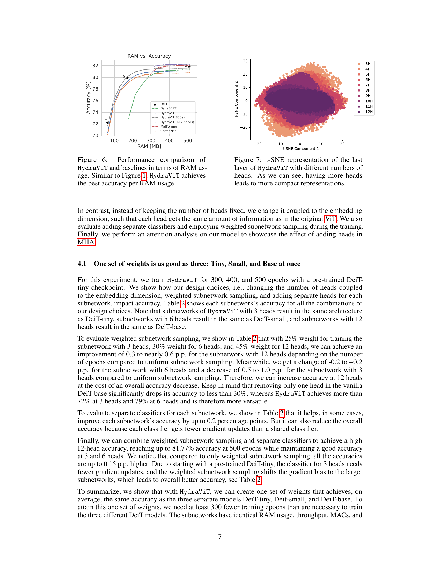
This figure compares the performance of HydraViT against several baseline models in terms of RAM usage and accuracy. It shows that HydraViT achieves superior accuracy for a given amount of RAM compared to other models like DeiT, DynaBERT, MatFormer, and SortedNet. This highlights HydraViT’s efficiency in resource-constrained environments. The figure plots accuracy on the y-axis and RAM usage in MB on the x-axis, clearly demonstrating HydraViT’s advantage.
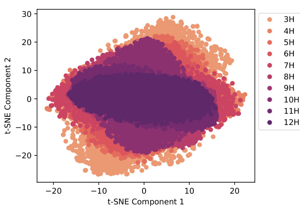
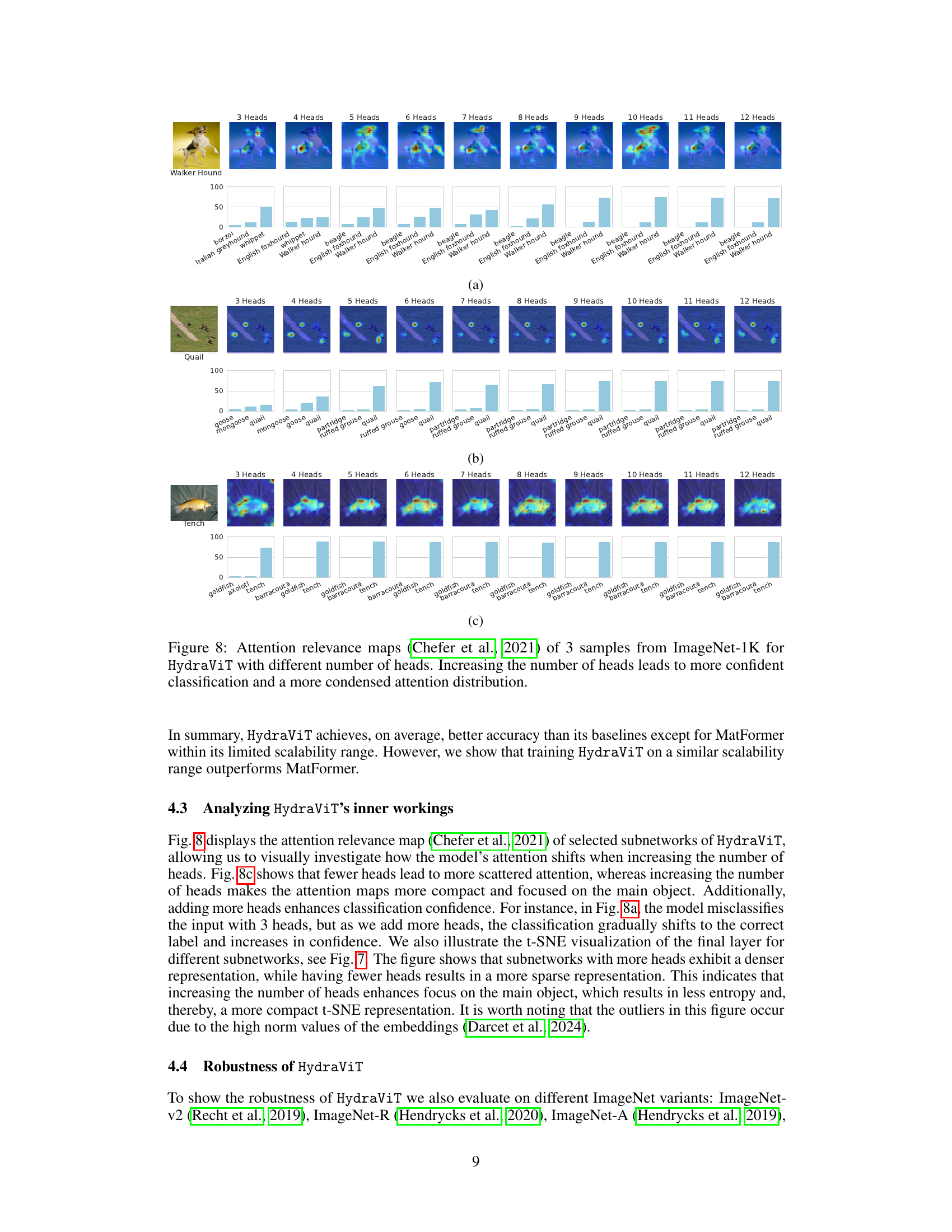
This figure shows a t-SNE (t-distributed Stochastic Neighbor Embedding) visualization of the feature representations from the last layer of the HydraViT model. Each point represents a data sample’s feature vector. The color of each point indicates the number of attention heads used in the corresponding HydraViT subnetwork (ranging from 3 to 12 heads). The visualization demonstrates that as the number of heads increases, the feature representations become more compact and clustered, suggesting improved representation efficiency and potentially better performance.

This figure compares the performance of HydraViT against several baselines (DeiT, DynaBERT, MatFormer, and SortedNet) on the ImageNet-1K dataset. The comparison is shown using two plots: one illustrating the relationship between GMACs (giga multiply-accumulate operations, a measure of computational complexity) and accuracy, and the other showing the relationship between throughput (images processed per second) and accuracy. The results demonstrate that HydraViT, particularly when trained with a wider range of heads (9-12), achieves higher accuracy for a given level of computational cost and throughput compared to the baselines.

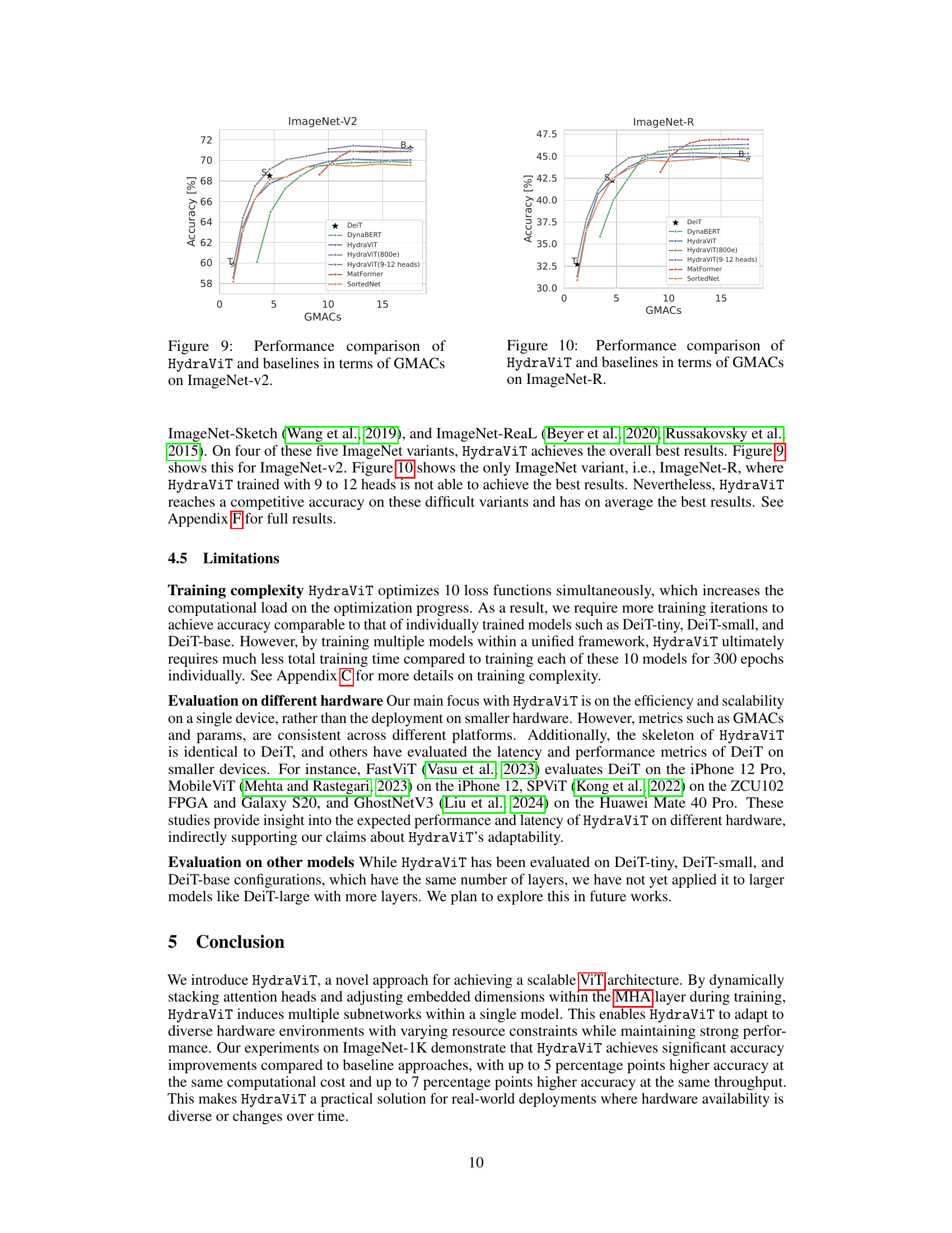
This figure shows the performance comparison of HydraViT and several baseline models (DeiT, DynaBERT, MatFormer, SortedNet) on the ImageNet-V2 dataset. The x-axis represents the number of GMACs (giga multiply-accumulate operations), a measure of computational cost, while the y-axis represents the accuracy achieved. The graph plots the accuracy of each model against its computational cost. It allows for comparison of the efficiency and accuracy trade-offs among different architectures. HydraViT is shown in multiple variations, indicating performance with different training epochs and a narrower head range. This illustrates how the model scales its performance based on resource constraints.
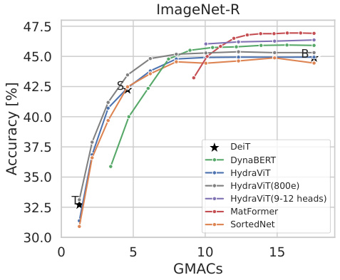
This figure compares the performance of HydraViT against several baseline models (DeiT, DynaBERT, MatFormer, SortedNet) on the ImageNet-R dataset. The comparison is made using GMACs (giga multiply-accumulate operations) as a measure of computational cost. Each line represents a different model, showing how accuracy varies with increasing computational complexity. HydraViT and its variants trained for 800 epochs and with a focus on 9-12 heads demonstrate competitive accuracy compared to other baselines, particularly in the lower GMAC range.
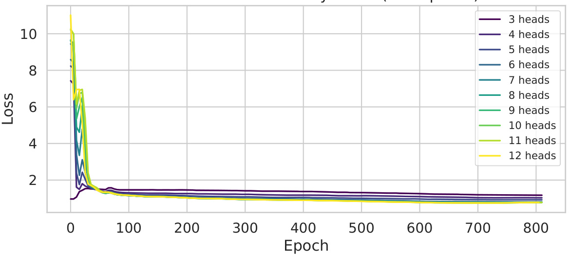
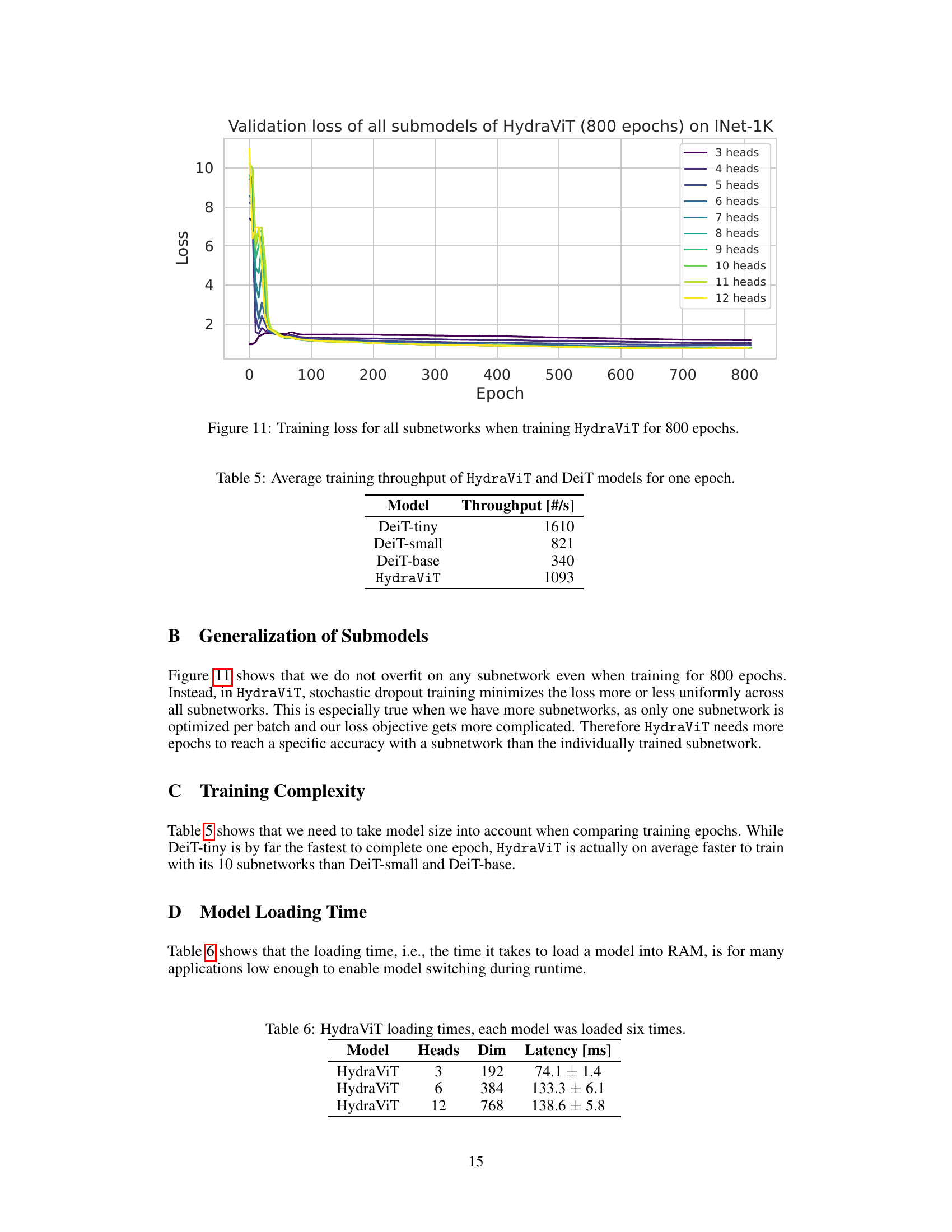
This figure shows the training loss curves for each subnetwork (3 to 12 heads) of HydraViT trained for 800 epochs. It demonstrates the training process of the model, showing how the loss decreases for each subnetwork over time. This illustrates that stochastic dropout training effectively minimizes the loss for all subnetworks, with no significant overfitting on any individual subnetwork even with the extensive training duration.

The figure presents a performance comparison of HydraViT against other models (DynaBERT, SortedNet, MatFormer, DeiT) on the ImageNet-1K dataset. It uses two graphs: one showing accuracy vs. GMACs (giga multiply-accumulate operations), and the other showing accuracy vs. throughput. HydraViT demonstrates better performance across various resource constraints, especially when trained with 9-12 heads.
More on tables
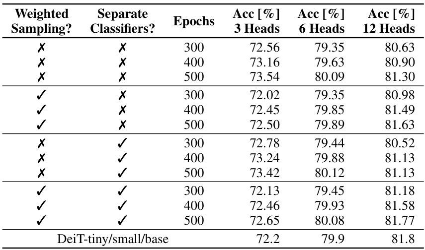
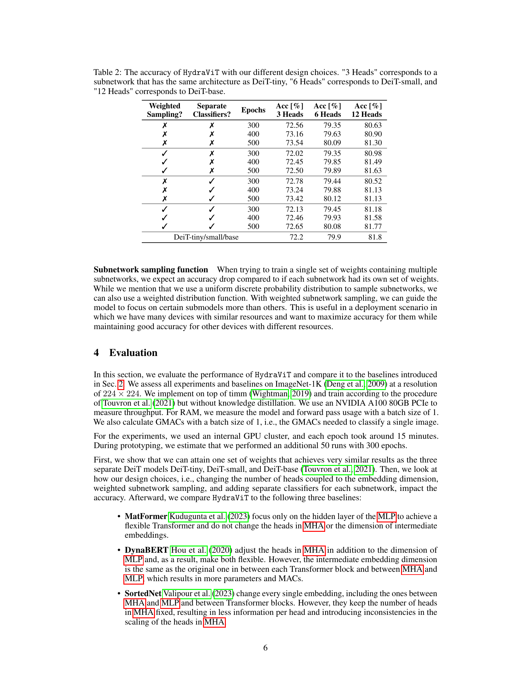
This table presents the accuracy results of HydraViT under various design choices. It investigates the impact of three factors on the model’s performance: weighted sampling of subnetworks during training, the use of separate classifier heads for each subnetwork, and the number of training epochs. The results are shown for three different subnetwork sizes, corresponding to the DeiT-tiny, DeiT-small, and DeiT-base models. Each row represents a specific configuration of these three factors, and the accuracies achieved for each subnetwork size are reported. The final row shows the accuracies of the original DeiT models for comparison.
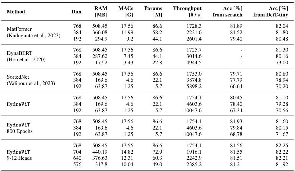
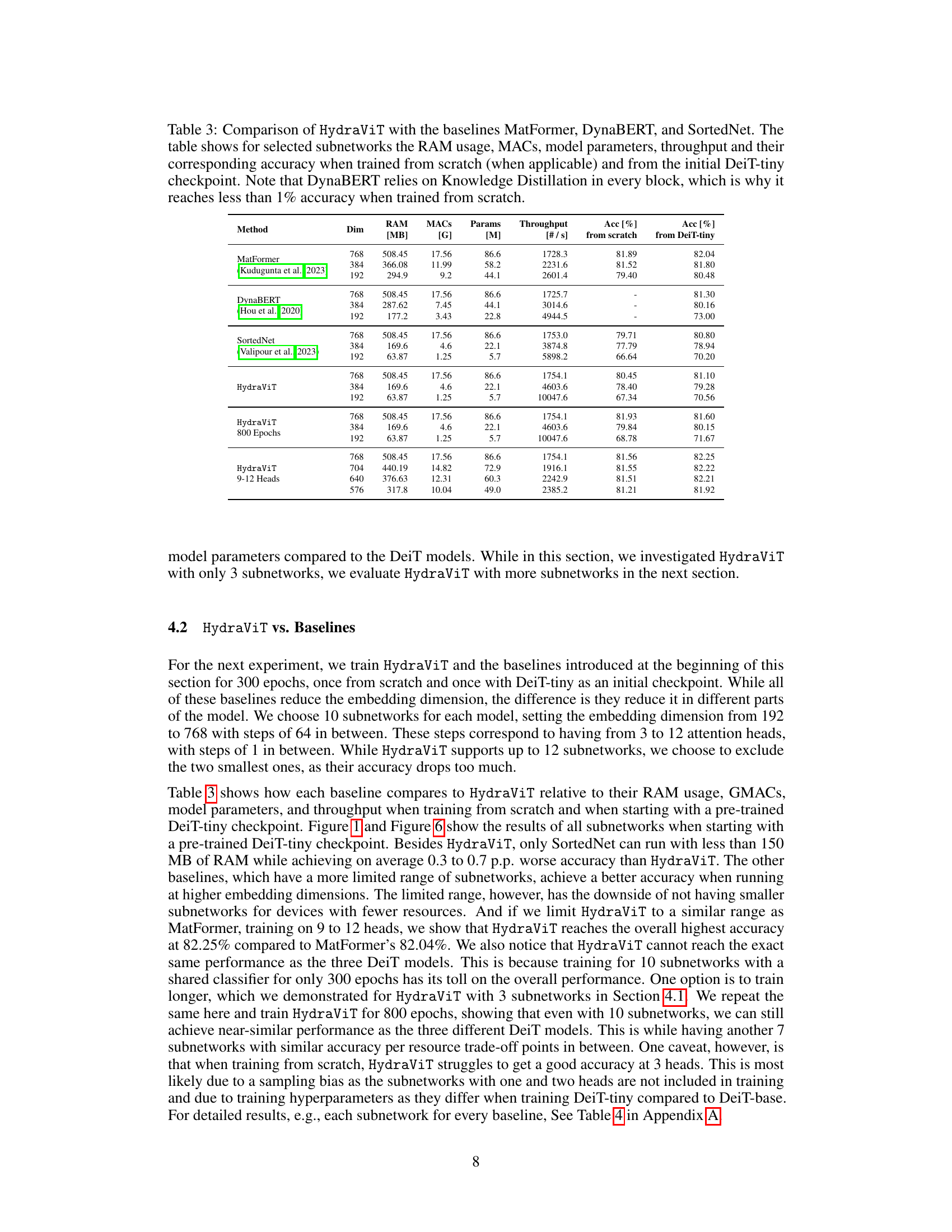
This table compares HydraViT against three baseline models (MatFormer, DynaBERT, and SortedNet) across different subnetwork sizes (defined by embedding dimension). It shows the RAM usage, number of Multiply-Accumulate operations (MACs), model parameters, throughput, and accuracy for each model, both when trained from scratch and initialized with a DeiT-tiny checkpoint. The table highlights HydraViT’s efficiency and performance relative to the baselines, especially when considering that DynaBERT uses knowledge distillation which gives it an unfair advantage when initialized with a checkpoint.
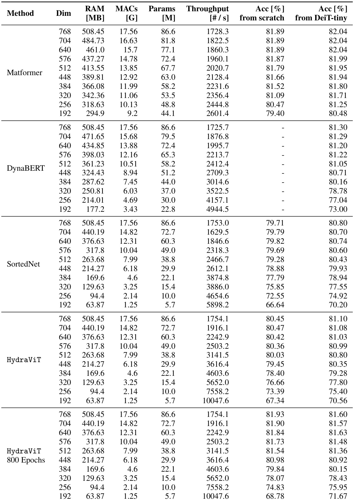
This table compares the performance of HydraViT against three baseline models (MatFormer, DynaBERT, and SortedNet) across various subnetworks. It provides key metrics for each model including RAM usage, number of Multiply-Accumulate operations (MACs), model parameters, throughput, and accuracy. The accuracy is shown for two training scenarios: training from scratch and training initialized with a DeiT-tiny checkpoint. A note highlights that DynaBERT’s reliance on Knowledge Distillation affects its accuracy when training from scratch.
This table compares the performance of HydraViT against three other models (MatFormer, DynaBERT, and SortedNet) across various metrics. It shows RAM usage, number of multiply-accumulate operations (MACs), model parameters, throughput, and accuracy for different subnetwork sizes. The comparison is made for models trained both from scratch and initialized using DeiT-tiny weights. A key observation is that DynaBERT’s performance suffers significantly when trained from scratch due to its reliance on knowledge distillation.

This table presents the latency results of loading different HydraViT models with varying numbers of heads and embedding dimensions. Each model was loaded six times to measure the latency, providing an average loading time and standard deviation for each configuration. This data helps demonstrate the model loading time of HydraViT, highlighting its efficiency and suitability for scenarios where switching models at runtime is necessary.

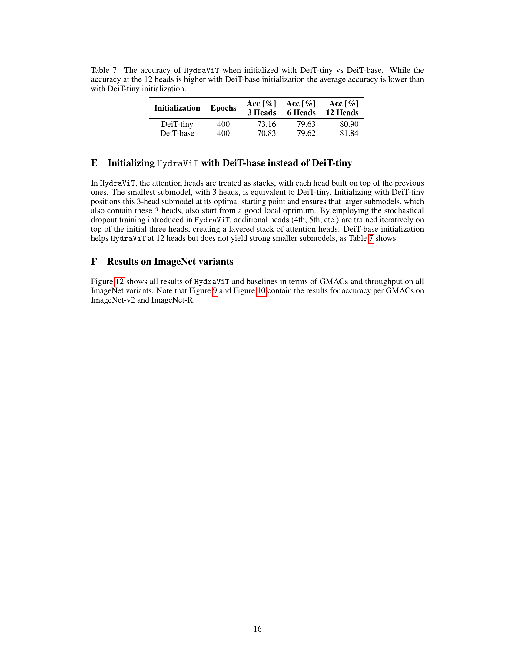
This table compares the accuracy of HydraViT when initialized with either DeiT-tiny or DeiT-base. It shows the accuracy achieved with 3, 6, and 12 heads after 400 epochs of training. While DeiT-base initialization leads to slightly better accuracy with 12 heads, the average accuracy across all three head configurations is superior when using DeiT-tiny initialization.
Full paper#


