↗ OpenReview ↗ NeurIPS Homepage ↗ Hugging Face ↗ Chat
TL;DR#
Molecular property prediction using Graph Neural Networks (GNNs) is a significant challenge. Current GNNs struggle to scale due to inefficiencies in sparse operations, large data demands, and unclear architectural effectiveness. This limits their application in fields like drug discovery which requires analyzing complex molecules. This research addresses these challenges by systematically investigating the scaling behavior of GNNs across various architectures. The work shows GNNs benefit immensely from increased model size, dataset size, and label diversity, especially when using a diverse pretraining dataset. This contrasts with previous findings that GNNs don’t benefit from scale.
The researchers introduce MolGPS, a new large-scale graph foundation model. MolGPS is trained using a diverse, large dataset and outperforms existing state-of-the-art models on many downstream tasks. This strongly supports the idea of scaling up GNNs for molecular property prediction, opening the door to significant advancements in drug discovery and materials science. The work paves the way for foundational GNNs to become a key driver of pharmaceutical drug discovery and molecular property prediction.
Key Takeaways#
Why does it matter?#
This paper is crucial because it addresses the critical need for scalable graph neural networks (GNNs) in molecular property prediction, a field currently hindered by computational limitations and data scarcity. The findings provide valuable insights into how model size, data diversity, and architecture impact performance, paving the way for more efficient and effective GNNs in drug discovery and other chemical applications. The introduction of MolGPS, a novel foundation model, demonstrates the substantial improvements possible through scaled-up models and refined training strategies. Furthermore, the research offers a strong foundation for future studies investigating the unique challenges of scaling GNNs and optimizing them for specific molecular tasks.
Visual Insights#
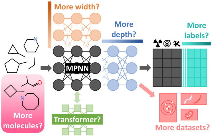
This figure summarizes the different scaling hypotheses tested in the paper. The authors investigated how varying the model width, depth, the number of molecules and labels in the training dataset, and the diversity of the datasets affected the performance of different GNN architectures (message-passing networks, graph transformers, and hybrid models). The baseline model is shown in dark gray, with variations in lighter colors representing the different scaling hypotheses.

This table compares the performance of different MolGPS variants (with and without phenomics data, and different model sizes) against the self-supervised GraphMVP model on the MoleculeNet benchmark. The test AUROC (Area Under the Receiver Operating Characteristic curve) is reported for four datasets (BACE, BBBP, Clintox, and Sider). Only datasets not used in the MolGPS pretraining are included in this comparison.
In-depth insights#
GNN Scaling Laws#
The exploration of GNN scaling laws in the context of molecular property prediction is insightful. The study reveals power-law relationships between model size, dataset size, and predictive performance, mirroring trends observed in other deep learning domains such as natural language processing and image generation. Crucially, the research demonstrates that increasing the model’s depth and width, along with the diversity and quantity of the training data (both molecules and their associated labels), leads to significant performance gains. This finding challenges previous assumptions about the limited scalability of GNNs for molecular tasks. The study highlights the importance of high-quality, diverse datasets for effective training, and that the choice of GNN architecture (MPNN, Transformer, Hybrid) plays a less significant role compared to the scale of these factors. The resulting model, MolGPS, showcases the potential for foundational GNN models in drug discovery and related fields. However, the study also acknowledges limitations including the need for further investigations into over-smoothing and data efficiency, particularly with deeper models.
MolGPS Model#
The MolGPS model, a foundational graph neural network (GNN) for molecular property prediction, represents a significant advancement in the field. Its core innovation lies in the scaling behavior demonstrated across various dimensions. This includes increasing model size (depth and width), dataset size (number of molecules), and label diversity (number of properties predicted per molecule). The model benefits tremendously from the diversity of its pretraining data, incorporating bioassays, quantum simulations, and more. MolGPS achieves state-of-the-art performance on various downstream tasks, showcasing the power of scaling GNNs in this specific domain. A key component of its success is the multi-fingerprint probing strategy, effectively leveraging learned representations from different model architectures and training phases. The inclusion of phenomic imaging data further enhances MolGPS’s predictive capabilities, highlighting the potential for multimodal data integration in future GNN models. While the study primarily focuses on supervised learning, the results pave the way for exploration of scaling in unsupervised GNN pretraining, which could unlock further progress in navigating complex chemical spaces.
Multi-task Learning#
Multi-task learning (MTL) in the context of molecular graph neural networks (GNNs) presents a powerful paradigm. By jointly learning multiple molecular properties from a shared representation, MTL leverages the inherent relationships between different tasks to improve overall predictive performance and efficiency. This contrasts with single-task learning, which trains separate models for each property, potentially leading to overfitting and higher computational costs. A key advantage of MTL for GNNs is its ability to address data scarcity issues common in molecular datasets. By training on a diverse range of tasks, the model learns a richer, more generalizable representation that can then be effectively transferred to new, unseen tasks. However, careful consideration must be given to task relatedness and potential negative transfer. Poorly chosen tasks might lead to interference and hinder performance, highlighting the critical role of dataset curation and task selection. Furthermore, the choice of architecture and training strategy significantly impact the effectiveness of MTL in this setting. Ultimately, successful implementation of MTL for GNNs in molecular property prediction promises more efficient and accurate models, accelerating drug discovery and materials science research.
Data Diversity#
Data diversity significantly impacts the performance of Graph Neural Networks (GNNs) in molecular property prediction. A larger variety of labels per molecule, sourced from diverse assays like bioassays, quantum simulations, and phenomic imaging, enhances the model’s ability to generalize and predict properties across a wider range of chemical space. Higher data diversity leads to more robust and powerful models, as they are exposed to a richer representation of chemical structures and their associated characteristics. This superior generalizability translates into better performance on downstream tasks, outperforming models trained on less diverse datasets. Therefore, investing in data diversity during the pretraining stage of GNNs is crucial for achieving superior performance in molecular property prediction.
Future Directions#
Future research could explore several promising avenues. Improving the efficiency of sparse operations within GNNs is crucial for better scalability. Investigating novel architectures or algorithmic optimizations tailored to the unique challenges of molecular graph processing is essential. Expanding the scope of pretraining datasets beyond the current limitations is key. This includes acquiring more data with high-quality labels across diverse molecular properties, integrating data from multiple modalities (e.g., combining phenomic imaging with bioassay data), and improving data curation techniques. Developing more effective self-supervised or semi-supervised training strategies for molecular GNNs is another critical area. Current methods struggle to capture the inherent complexity of molecular interactions. Researching new evaluation benchmarks beyond standard datasets is also needed to properly assess the capabilities of GNNs in real-world applications. A rigorous benchmark reflecting the full diversity of drug discovery tasks would greatly benefit the community.
More visual insights#
More on figures
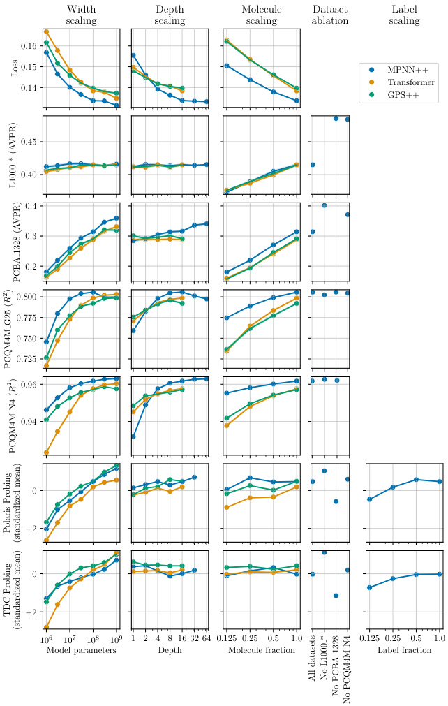
This figure shows the results of scaling experiments on various aspects of the GNN models, including width, depth, number of molecules, and labels, as well as dataset diversity. The different scaling methods are shown as columns, and the performance metrics are shown in rows. Each point represents the average standardized performance across multiple tasks. This illustrates the impact of these factors on model performance for various molecular tasks.
This figure shows the effects of scaling different aspects of the GNN models (width, depth, number of molecules, and number of labels) on model performance. Each row represents a different performance metric (e.g., AUROC, MAE) and each column shows a different scaling factor. The results demonstrate a positive scaling trend across all metrics for all scaling factors. The impact of each scaling factor is also shown.
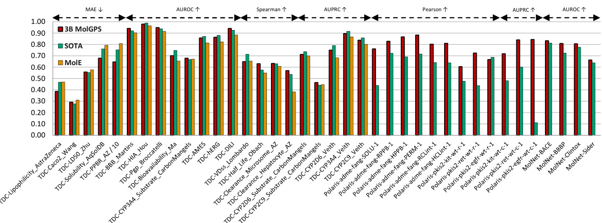
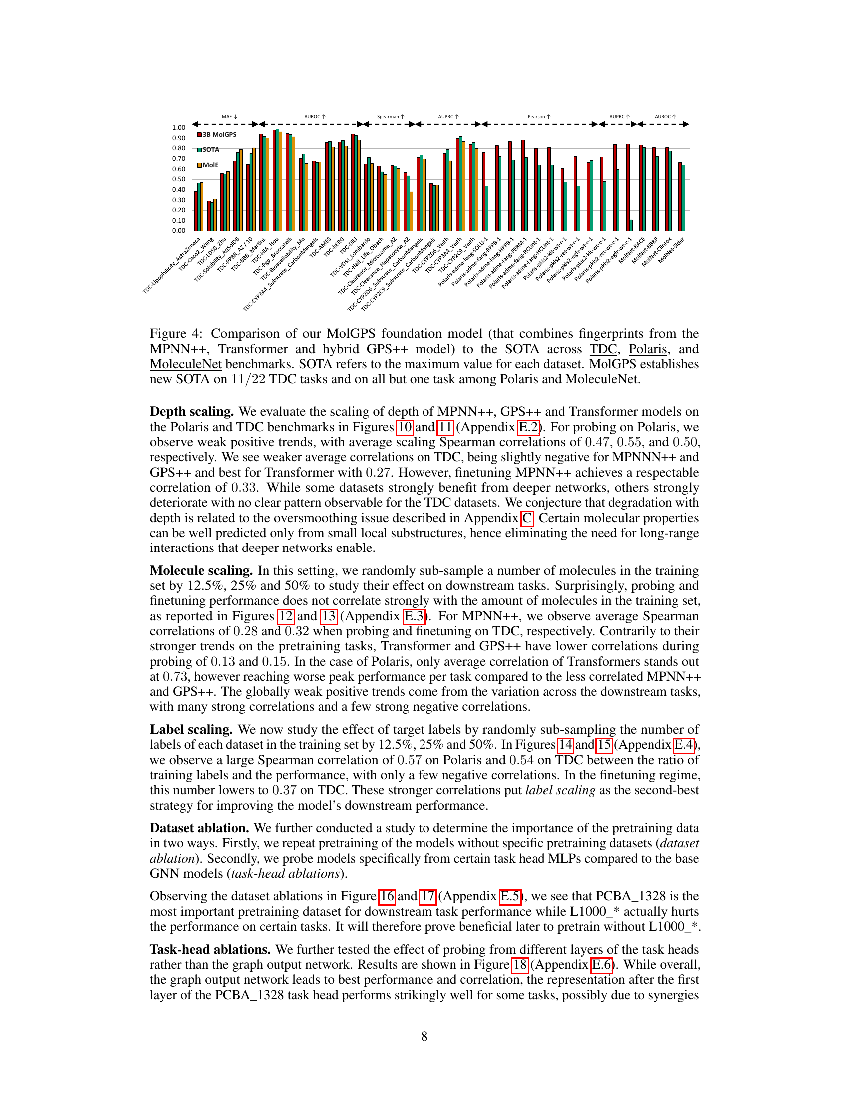
This figure compares the performance of the MolGPS model to the state-of-the-art (SOTA) across three benchmark datasets: TDC, Polaris, and MoleculeNet. MolGPS is a foundation model that combines fingerprints from three different architectures (MPNN++, Transformer, and hybrid GPS++). The figure shows that MolGPS achieves SOTA performance on a significant portion of the tasks in each dataset, demonstrating its effectiveness as a general-purpose model for various molecular property prediction tasks.
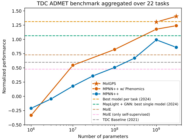
This figure compares the performance of three different models (MPNN++, MPNN++ with phenomics, and MolGPS) on the TDC ADMET benchmark. The x-axis represents the number of parameters in each model, and the y-axis represents the normalized performance across the 22 tasks in the benchmark. The figure shows that MolGPS significantly outperforms the other models, demonstrating strong scaling behavior and the benefit of incorporating phenomics data into the pretraining process. Several baselines are also included for comparison, showing the relative performance improvements of the presented models.
This figure presents the results of an experiment that investigates the scaling behavior of Graph Neural Networks (GNNs) for molecular graphs in various settings. Different columns explore different scaling factors (width, depth, number of molecules, datasets, labels) while rows show different performance metrics. The standardized mean metric is used for better comparison across various tasks.
This figure shows the effects of scaling different aspects of the models and datasets on their performance. The rows represent the different performance metrics used, and the columns represent the different aspects being scaled (width, depth, number of molecules, datasets, labels). Each point shows the average standardized performance across multiple tasks. The lighter colors indicate better performance.

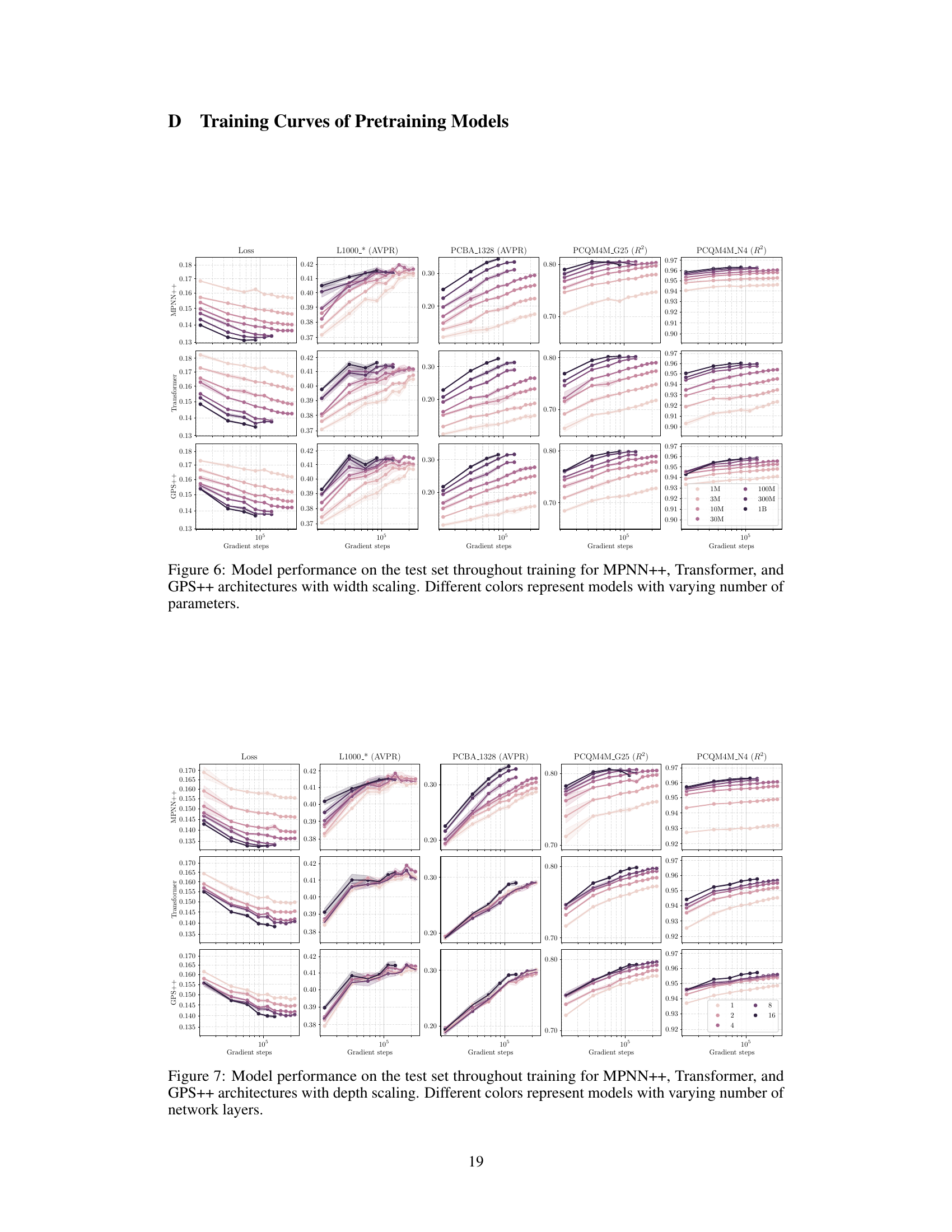
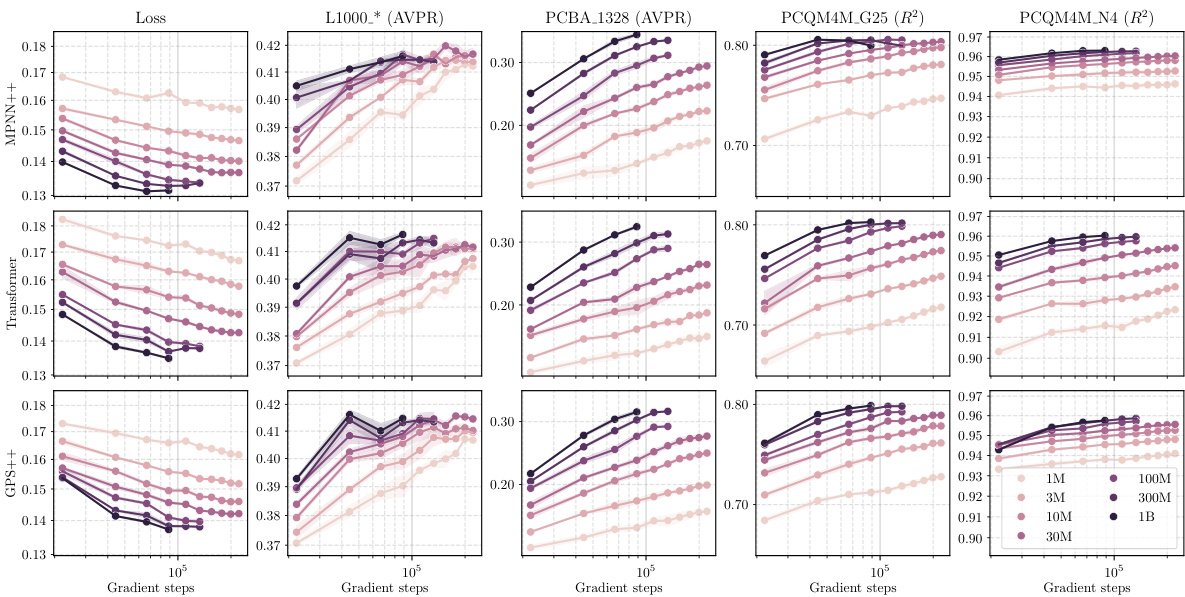
This figure shows the training curves for three different GNN architectures (MPNN++, Transformer, and GPS++) while varying the fraction of molecules used for training. The x-axis represents the number of gradient steps, and the y-axis shows the loss for the different datasets used for pretraining. Each line represents a model trained with a different fraction of the total dataset (12.5%, 25%, 50%, 100%). The figure illustrates how the model performance and training loss change with different amounts of training data and the different GNN architectures.

This figure shows the results of experiments evaluating how different scaling factors affect the performance of various GNN models. The rows represent different performance metrics (e.g., standardized mean for various tasks), and columns show the impact of different scaling factors like width, depth, molecule count, and dataset diversity. The lighter and darker shades of green indicate better and worse performances respectively. The figure helps to visualize which scaling methods have the greatest effect on improving model performance for specific tasks.

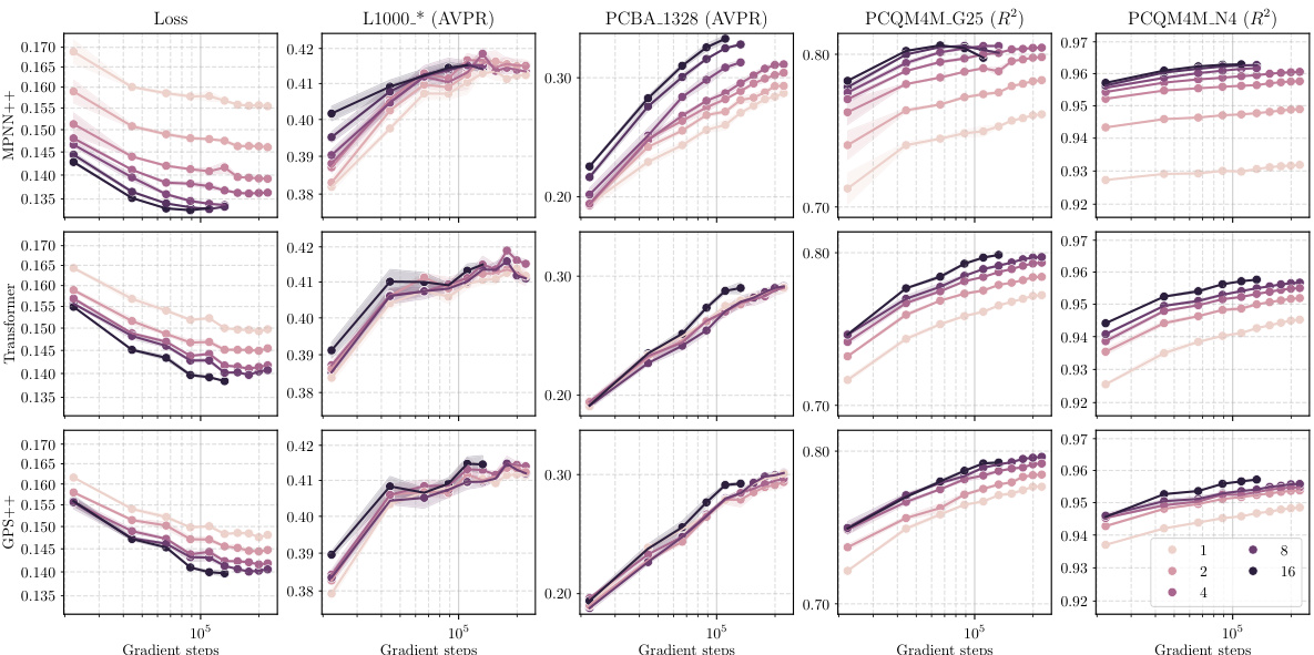
This figure shows the results of scaling experiments on molecular GNNs. It analyzes how performance changes with variations in model width, depth, number of molecules, labels, and dataset diversity. Different rows show different performance metrics. Different columns show the effects of varying the different scaling factors (width, depth, molecules, dataset, labels). The graphs illustrate the scaling behavior of three different GNN architectures (MPNN++, Transformer, and GPS++) across multiple datasets and tasks.

This figure shows the impact of scaling different aspects of the model and data on the performance across various tasks. It shows scaling with respect to the model’s width (number of parameters), depth (number of layers), the number of molecules in the dataset, the diversity of datasets used, and the number of labels per molecule. Different colors represent different model architectures (MPNN++, Transformer, and GPS++). The y-axis represents the average standardized performance across different tasks. Each column represents a different scaling factor, and each row represents a different performance metric.

This figure shows the effects of scaling on the performance of different GNN architectures. Each column represents a scaling type (width, depth, number of molecules, dataset ablation, label scaling), and each row represents a performance metric. The standardized mean is shown, which normalizes performance scores across various tasks. The results demonstrate how changes in model size and dataset affect performance on different tasks, illustrating power law scaling behavior. For example, increasing the model width significantly improves performance, while increasing the depth has diminishing returns after a certain point.

This figure shows the results of scaling experiments on various aspects of the GNN models. The rows represent different performance metrics (e.g., AUROC, R-squared), while the columns represent different scaling factors (e.g., width, depth, number of molecules, dataset diversity, and number of labels). Each cell in the figure shows the standardized mean performance across multiple tasks, which allows for a comparison of scaling effects across different metrics and factors. The use of a standardized mean allows for comparisons even though the datasets involved had different scoring systems.

This figure summarizes the different scaling hypotheses explored in the paper. It shows how the authors investigated scaling graph neural networks (GNNs) by varying several key factors, including the model’s width (number of parameters), depth (number of layers), the size of the molecular dataset (number of molecules), the number of labels per molecule, and the diversity of the datasets. The baseline model is represented in dark grey, while variations are shown in lighter colors.

This figure shows the results of scaling experiments on molecular GNNs. Different scaling types (width, depth, number of molecules, dataset ablation, label fraction) were tested, and their effects on various downstream tasks are shown. The standardized mean performance across tasks is presented, providing a summary of the scaling behaviors for different GNN architectures (MPNN++, Transformer, GPS++).
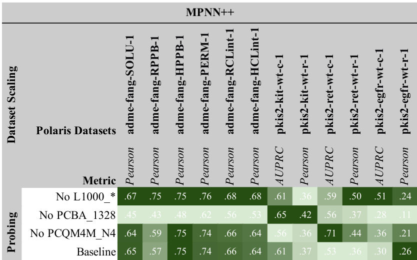
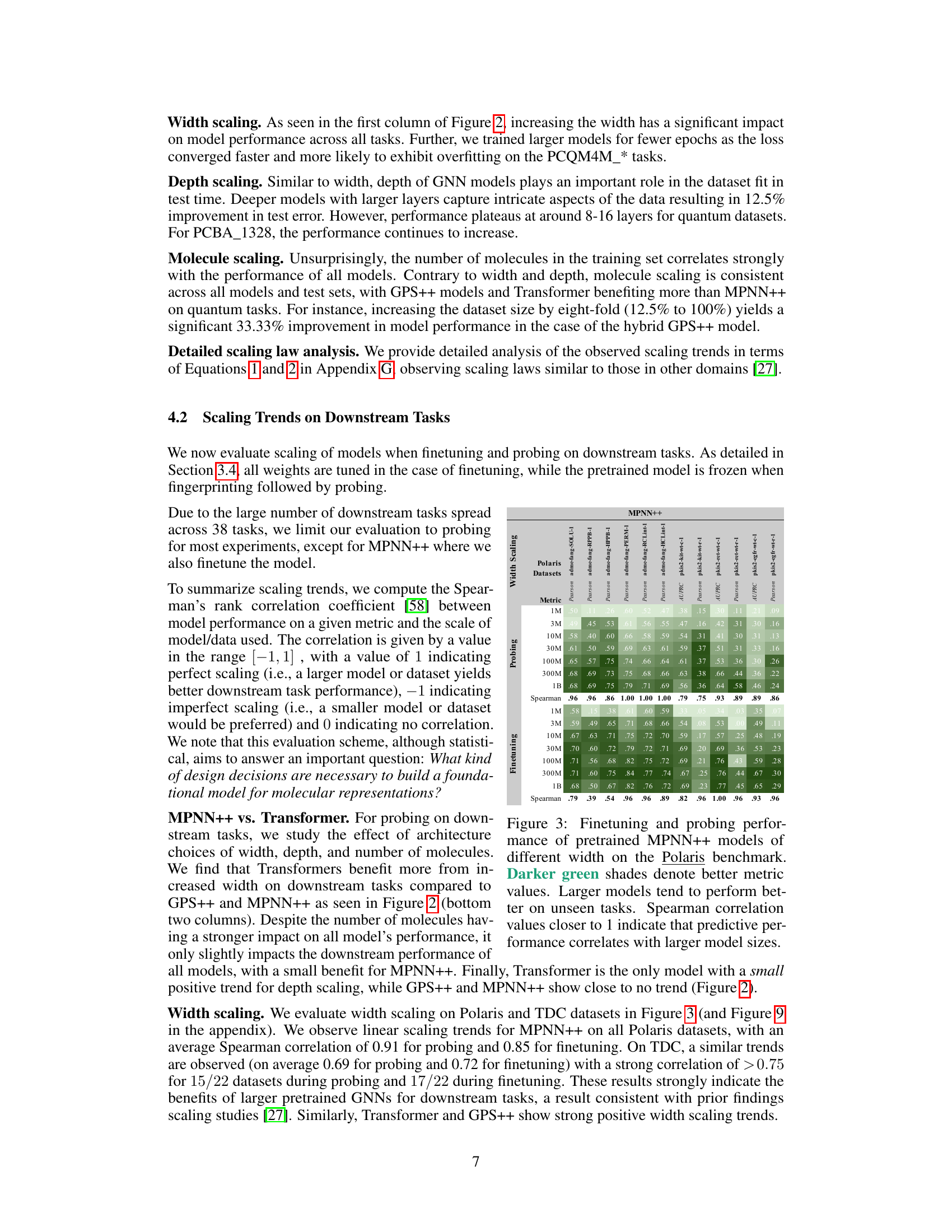
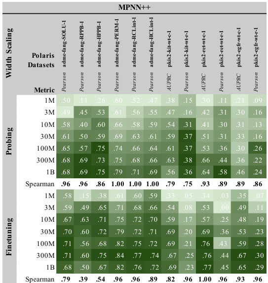
This figure shows the results of scaling experiments on the TDC benchmark dataset for three different GNN architectures (MPNN++, Transformer, and GPS++). It demonstrates the impact of increasing model width (number of parameters) on model performance, evaluated using both probing and finetuning strategies. Darker green indicates better performance. The Spearman correlation values quantify the strength of the relationship between model size and performance for both probing and finetuning. This provides evidence that model size is an important factor in achieving better results.

This figure displays the results of scaling experiments on various factors including width, depth, number of molecules, dataset size, and the number of labels. Each row represents a different performance metric (e.g., AUPRC, Spearman, MAE), and each column a different scaling approach. The graphs show how these changes affect performance on different downstream tasks, providing insights into how molecular GNNs scale.
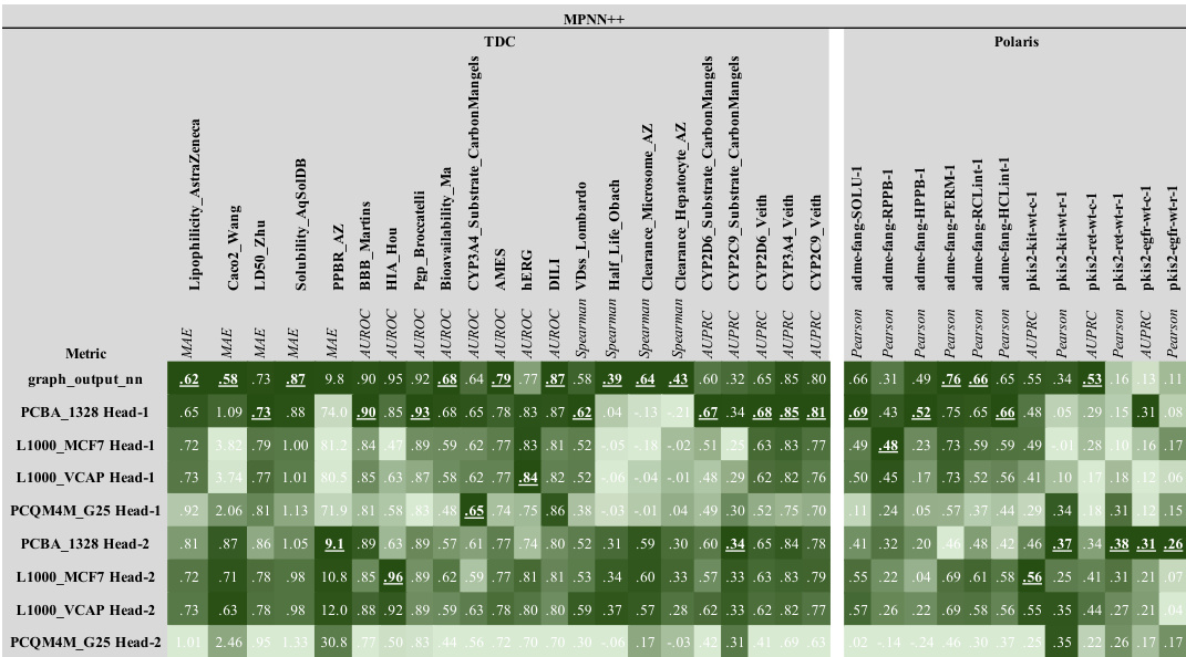
This figure shows the results of scaling experiments on molecular GNNs. It explores how changes in model width, depth, dataset size, and number of labels affect performance across various tasks (L1000, PCBA, PCQM4M). Each row represents a performance metric, and each column shows a different scaling factor. The standardized mean performance is shown for each condition, providing a comprehensive view of the scaling behavior for different GNN architectures (MPNN++, Transformer, GPS++).
More on tables

This table compares the performance of MolGPS variants (with and without phenomics data) against the self-supervised and fully supervised versions of the MolE model. The comparison is performed on the TDC benchmark dataset, and focuses on normalized MAE scores for various tasks. The results highlight that supervised pretraining greatly improves MolE’s performance, and MolGPS consistently surpasses all MolE versions across most tasks.

This table presents the power law constants (α) obtained from applying Equation 1 to the results of the width scaling experiments on the Polaris benchmark (shown in Figure 3). These constants represent how much the loss function changes with respect to changes in model parameters, specifically for different downstream tasks (T1-T12). The values are shown separately for probing and finetuning strategies, demonstrating differences in how model scaling impacts performance based on the training approach.

This table shows the power-law scaling behavior of different GNN architectures (MPNN++, Transformer, and GPS++) during pretraining. It presents the power-law constant (β) obtained from Equation 2, which relates the training loss to the dataset size. The values of β indicate how efficiently the models use the increasing amount of training data. Higher β values suggest better scaling behavior.
Full paper#


