TL;DR#
Dynamic Bayesian Optimization (DBO) faces challenges managing data efficiently as the objective function changes over time. Existing methods either reset the dataset periodically or assign decreasing weights to old observations, which can lead to suboptimal performance. This paper introduces the W-DBO algorithm, which uses a novel criterion based on the Wasserstein distance to quantify the relevance of each observation, and selectively removes stale data. This technique allows maintaining predictive accuracy and high sampling frequency while managing dataset size effectively.
The core of W-DBO is a new criterion which leverages the Wasserstein distance to measure the impact of removing an observation on future predictions. Using this criterion, W-DBO efficiently removes irrelevant observations in an online setting. The algorithm’s performance is evaluated through numerical experiments, demonstrating that W-DBO consistently outperforms state-of-the-art methods, leading to a significant improvement in both predictive accuracy and computational efficiency. This makes W-DBO highly relevant for practical applications of DBO where computational cost and real-time performance are crucial.
Key Takeaways#
Why does it matter?#
This paper is crucial for researchers in Bayesian Optimization and related fields because it directly addresses the limitations of existing dynamic Bayesian optimization (DBO) methods. W-DBO’s efficient data management strategy is particularly important for continuous-time optimization tasks with unknown horizons, a very common scenario in real-world applications. The new Wasserstein distance-based criterion for quantifying observation relevance opens exciting new avenues for improving DBO algorithms and extends their applicability to a wider range of problems.
Visual Insights#
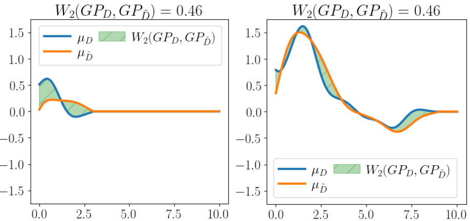
🔼 This figure compares two pairs of posterior Gaussian processes (GPs). Each pair has the same 2-Wasserstein distance (0.46), which quantifies the difference between the two distributions. However, the left pair shows GPs that are very similar while the right pair shows GPs that are very different. This illustrates how the length scale of the GP significantly influences the shape of the posterior distribution even when the overall Wasserstein distance remains constant.
read the caption
Figure 1: Similar values of Wasserstein distance, different effect on posteriors. For visualization purposes, only the posterior means of two posterior GPs (blue for μD and orange for μD) are depicted, along a single dimension (e.g., time). The Wasserstein distance between the two posteriors is shown by the green shaded area. The GPs have a small lengthscale (left) or, conversely, a large lengthscale (right) for the chosen dimension.

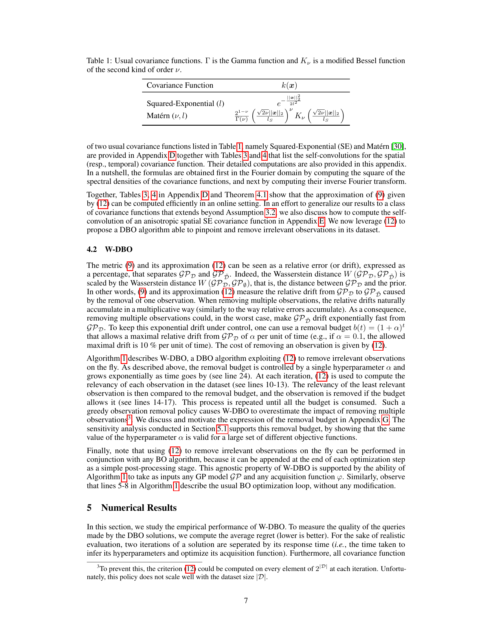
🔼 This table shows the mathematical formulas for two commonly used covariance functions in Gaussian processes: the Squared-Exponential and the Matérn. These functions are used to model the correlation between different data points in a dataset. The formulas include parameters like lengthscale (l) which controls the smoothness and range of correlation and v which affects the smoothness of the Matérn function. These are crucial in Bayesian Optimization for modeling the objective function and are thus vital to understanding the W-DBO algorithm performance.
read the caption
Table 1: Usual covariance functions. Γ is the Gamma function and K, is a modified Bessel function of the second kind of order v.
In-depth insights#
Stale Data Removal#
The concept of stale data removal is crucial in dynamic Bayesian Optimization (DBO) because the objective function changes over time. Observations made earlier become less relevant for predicting the optimum in the future. The paper introduces a method to quantify this irrelevance using a Wasserstein distance-based criterion, which measures the difference in the Gaussian Process (GP) posterior distribution after removing an observation. This criterion helps identify stale data points by calculating a relevancy score. A low score indicates that removing the observation has minimal impact on future predictions. This efficient criterion allows W-DBO to remove irrelevant data online, balancing predictive performance and computational cost. The removal strategy efficiently maintains a high sampling frequency even in scenarios with continuous-time optimization, thus preventing the dataset size from growing excessively and improving the algorithm’s response time. The effectiveness of this approach is demonstrated in the numerical results, showing W-DBO’s superiority over existing methods in dynamic optimization tasks.
W-DBO Algorithm#
The W-DBO algorithm innovatively addresses the challenge of stale data in dynamic Bayesian optimization (DBO). It leverages a Wasserstein distance-based criterion to quantify the relevancy of each observation. This allows the algorithm to efficiently remove irrelevant data points, thereby maintaining good predictive performance while enabling a high sampling frequency. The algorithm’s ability to adapt on-the-fly, removing stale observations while preserving crucial information, distinguishes it from other DBO methods. This is particularly crucial for continuous-time optimization with unknown horizons. The use of a removal budget further enhances its practicality, balancing data reduction with maintaining predictive accuracy. While computational tractability is addressed through approximations, the overall effectiveness of W-DBO, as demonstrated in numerical experiments, showcases its significant advantage in handling dynamic optimization tasks.
Wasserstein Distance#
The concept of “Wasserstein Distance” within the context of a research paper likely revolves around quantifying the similarity between probability distributions. In the specific application of Bayesian Optimization, it’s used to measure the relevance of past observations in a dynamic environment. Instead of simply discarding old data points, the Wasserstein distance helps determine which observations are still informative for predicting the future optimum. This approach is powerful because it avoids discarding potentially valuable information too soon. The method’s efficiency stems from providing a way to dynamically manage the dataset, ensuring that the computational cost remains reasonable even with continuous-time optimization. By selectively removing stale data, it’s possible to maintain a high sampling frequency and high predictive performance, which are normally conflicting goals in dynamic Bayesian optimization. Therefore, the use of Wasserstein distance is crucial for improving both efficiency and accuracy in this context.
Computational Cost#
The computational cost of Bayesian Optimization (BO) algorithms, especially in dynamic settings, is a critical concern. Standard BO methods have a time complexity that scales cubically with the dataset size, making them impractical for high-frequency data acquisition in dynamic environments. The paper addresses this by introducing a novel criterion to quantify the relevancy of observations and a method to efficiently remove stale data. This significantly reduces the computational burden, allowing for higher sampling frequency and improved tracking of the optimum in dynamic systems. While the proposed method still involves matrix inversions, its efficiency gains are achieved by focusing on the most relevant data points. Approximations and upper bounds are used to reduce computational cost. The practicality of the proposed algorithm depends heavily on the efficacy of these approximations; further analysis of approximation error and sensitivity to parameters is necessary for a full understanding of the computational performance. The online nature of the approach is a key advantage, enabling efficient operation in dynamic contexts where data streams continuously arrive.
Future Research#
Future research directions stemming from this work on stale observation removal in dynamic Bayesian Optimization (DBO) are manifold. Extending the Wasserstein distance-based criterion to a broader class of covariance functions beyond the currently assumed spatio-temporal decomposable structure is crucial. This would enhance the applicability of the method to a wider range of real-world dynamic optimization problems. Further investigation into the theoretical guarantees, such as regret bounds, for the proposed W-DBO algorithm in continuous time settings is needed. Empirical analysis on more diverse and complex real-world datasets is vital, showcasing the robustness and practical advantages of W-DBO in varied applications. Finally, exploring the integration of W-DBO with other advanced BO techniques, like parallel or multi-objective BO, offers exciting avenues to push the boundaries of efficient and adaptive optimization in dynamic environments.
More visual insights#
More on figures
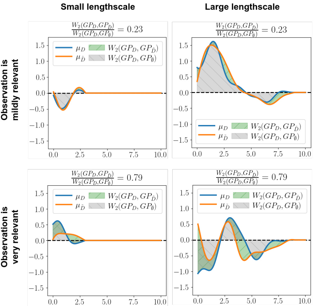
🔼 This figure shows the effect of the lengthscale parameter on the Wasserstein distance between two Gaussian Process (GP) posterior distributions. Two pairs of GP posteriors are displayed, each with a similar Wasserstein distance. However, the left pair, generated with a small lengthscale, displays similar posterior means, while the right pair, with a large lengthscale, exhibits significantly different means. The shaded area visually represents the Wasserstein distance between the posteriors in each case.
read the caption
Figure 1: Similar values of Wasserstein distance, different effect on posteriors. For visualization purposes, only the posterior means of two posterior GPs (blue for μD and orange for μD) are depicted, along a single dimension (e.g., time). The Wasserstein distance between the two posteriors is shown by the green shaded area. The GPs have a small lengthscale (left) or, conversely, a large lengthscale (right) for the chosen dimension.

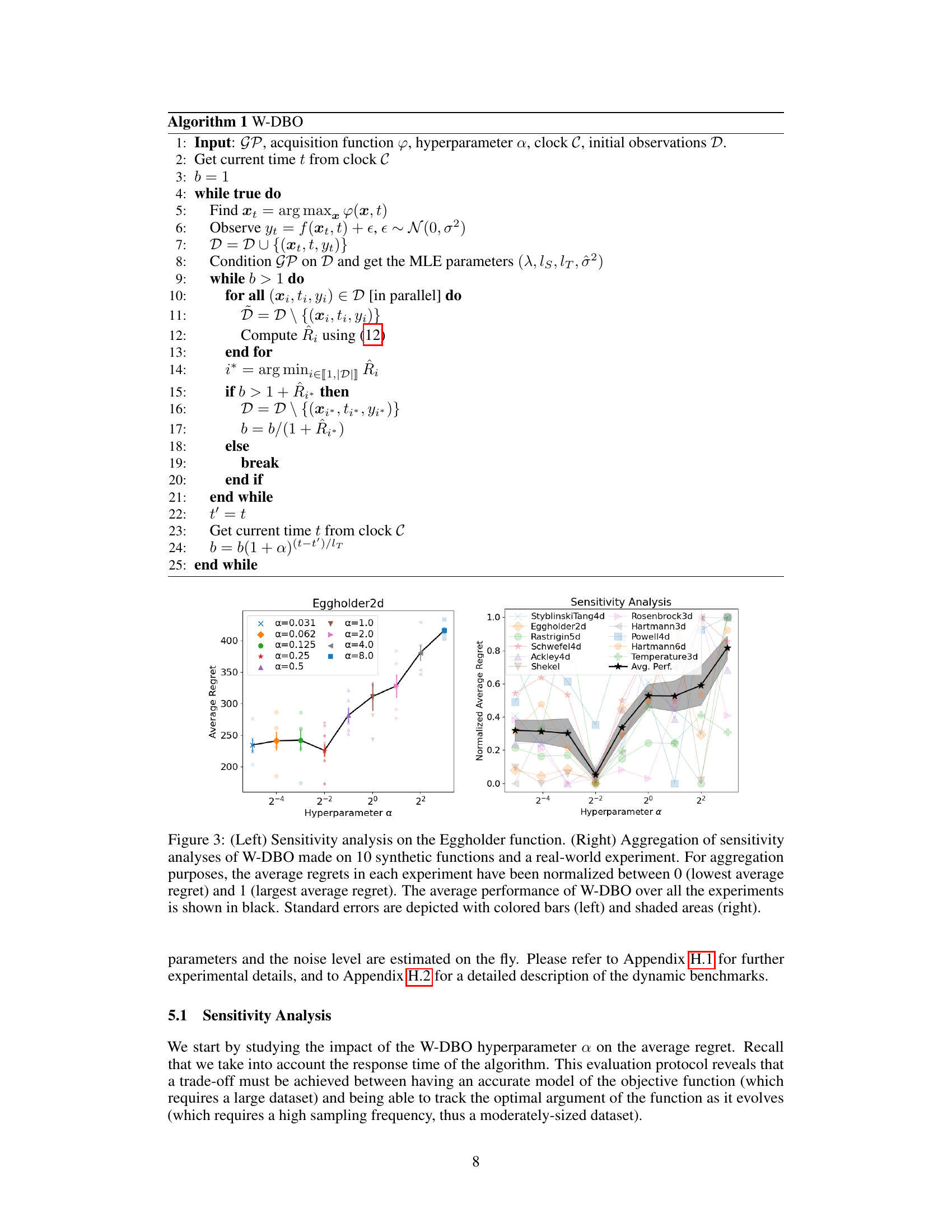
🔼 The left plot shows the sensitivity analysis of the hyperparameter α in the W-DBO algorithm on the Eggholder function. The right plot shows the aggregation of sensitivity analyses across multiple synthetic functions and a real-world experiment. It demonstrates how the average regret of W-DBO is impacted by changes in α. Standard errors are included to show uncertainty in the results.
read the caption
Figure 3: (Left) Sensitivity analysis on the Eggholder function. (Right) Aggregation of sensitivity analyses of W-DBO made on 10 synthetic functions and a real-world experiment. For aggregation purposes, the average regrets in each experiment have been normalized between 0 (lowest average regret) and 1 (largest average regret). The average performance of W-DBO over all the experiments is shown in black. Standard errors are depicted with colored bars (left) and shaded areas (right).
🔼 The left plot shows the sensitivity analysis of the hyperparameter α on the Eggholder function. The right plot aggregates the sensitivity analysis results of α across 10 different synthetic functions and one real-world experiment. The average regrets are normalized for easy comparison. The results show that W-DBO achieves the best performance with α=1.
read the caption
Figure 3: (Left) Sensitivity analysis on the Eggholder function. (Right) Aggregation of sensitivity analyses of W-DBO made on 10 synthetic functions and a real-world experiment. For aggregation purposes, the average regrets in each experiment have been normalized between 0 (lowest average regret) and 1 (largest average regret). The average performance of W-DBO over all the experiments is shown in black. Standard errors are depicted with colored bars (left) and shaded areas (right). parameters and the noise level are estimated on the fly.

🔼 This figure provides a visual summary of the results presented in Table 2. The average regrets for each experiment, across different DBO algorithms (GP-UCB, ABO, ET-GP-UCB, R-GP-UCB, TV-GP-UCB, and W-DBO), have been normalized to a range of 0 to 1 for easier comparison. The average performance across all experiments is shown in black, offering a concise overview of W-DBO’s performance relative to other algorithms.
read the caption
Figure 5: Visual summary of the results reported in Table 2. For aggregation purposes, the average regrets in each experiment have been normalized between 0 (lowest average regret) and 1 (largest average regret). The average performance of the DBO solutions is shown in black.
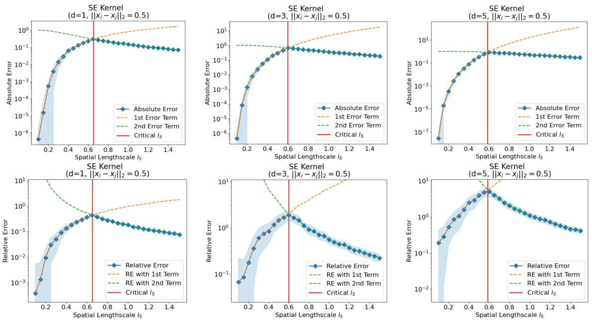
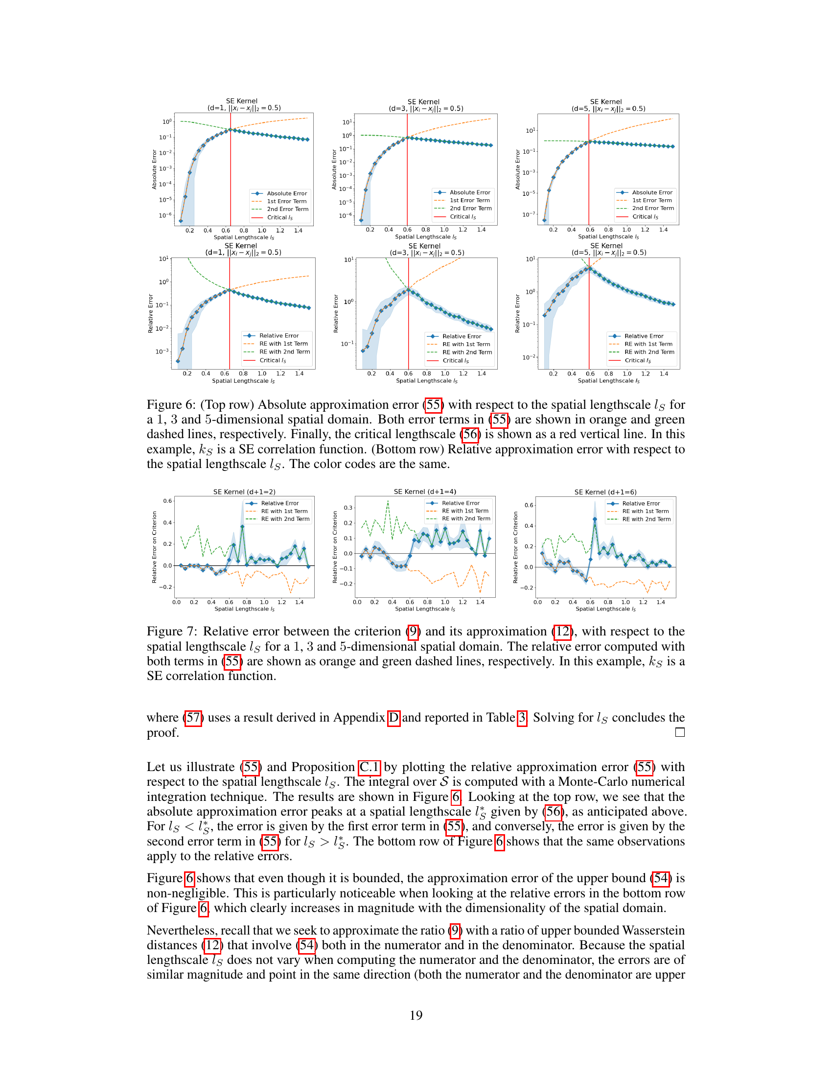
🔼 This figure shows the absolute and relative approximation errors of equation (55) for different spatial dimensions (1, 3, and 5). The top row displays the absolute error, while the bottom row shows the relative error. Both plots show the individual errors from the first and second terms in equation (55) and the overall error. The critical length scale is marked by a red line. The figure illustrates how the approximation error varies with the spatial lengthscale and dimension.
read the caption
Figure 6: (Top row) Absolute approximation error (55) with respect to the spatial lengthscale ls for a 1, 3 and 5-dimensional spatial domain. Both error terms in (55) are shown in orange and green dashed lines, respectively. Finally, the critical lengthscale (56) is shown as a red vertical line. In this example, ks is a SE correlation function. (Bottom row) Relative approximation error with respect to the spatial lengthscale ls. The color codes are the same.

🔼 This figure shows the absolute and relative approximation errors for equation (55) in the paper. The approximation error is plotted against the spatial lengthscale (ls) for 1, 3, and 5-dimensional spatial domains. The figure helps to visualize how the approximation error varies with the lengthscale and dimensionality, highlighting a critical lengthscale where the error is maximal.
read the caption
Figure 6: (Top row) Absolute approximation error (55) with respect to the spatial lengthscale ls for a 1, 3 and 5-dimensional spatial domain. Both error terms in (55) are shown in orange and green dashed lines, respectively. Finally, the critical lengthscale (56) is shown as a red vertical line. In this example, ks is a SE correlation function. (Bottom row) Relative approximation error with respect to the spatial lengthscale ls. The color codes are the same.
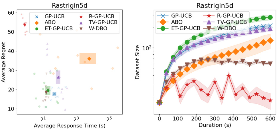
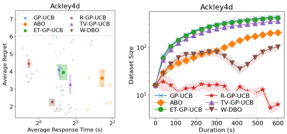
🔼 This figure shows the performance comparison of different Dynamic Bayesian Optimization (DBO) algorithms on the Rastrigin function. The left panel displays the average response time against the average regret, while the right panel illustrates the dataset size over time. This provides insights into the trade-off between computational cost (response time and dataset size) and optimization performance (regret).
read the caption
Figure 8: (Left) Average response time and average regrets of the DBO solutions during the optimization of the Rastrigin synthetic function. (Right) Dataset sizes of the DBO solutions during the optimization of the Rastrigin synthetic function.

🔼 This figure shows the performance comparison of different Dynamic Bayesian Optimization (DBO) algorithms on the Schwefel function. The left panel displays the average response time against the average regret, indicating the trade-off between computational cost and optimization performance. The right panel shows the dataset size of each algorithm over time, highlighting how the algorithms manage data over the optimization process. The results illustrate the performance differences between various DBO algorithms in terms of both accuracy and computational efficiency.
read the caption
Figure 9: (Left) Average response time and average regrets of the DBO solutions during the optimization of the Schwefel synthetic function. (Right) Dataset sizes of the DBO solutions during the optimization of the Schwefel synthetic function.

🔼 The left plot shows the average response time and average regret for different DBO algorithms on the Schwefel function. The right plot displays the dataset size of each algorithm over time. The figure illustrates the tradeoff between response time (dataset size) and optimization performance for various DBO methods.
read the caption
Figure 9: (Left) Average response time and average regrets of the DBO solutions during the optimization of the Schwefel synthetic function. (Right) Dataset sizes of the DBO solutions during the optimization of the Schwefel synthetic function.

🔼 This figure shows the performance of different DBO algorithms on the Styblinski-Tang function. The left panel shows the average response time against the average regret, indicating the trade-off between computational cost and optimization performance. The right panel displays the dataset size over time for each algorithm, highlighting how the size of the dataset used by each algorithm changes during the optimization process. This illustrates the impact of different strategies on dataset management. The algorithms compared include GP-UCB, ABO, ET-GP-UCB, R-GP-UCB, TV-GP-UCB, and W-DBO.
read the caption
Figure 11: (Left) Average response time and average regrets of the DBO solutions during the optimization of the Styblinski-Tang synthetic function. (Right) Dataset sizes of the DBO solutions during the optimization of the Styblinski-Tang synthetic function.
🔼 The left plot shows the sensitivity analysis of the W-DBO algorithm on the Eggholder function by varying the hyperparameter α. The right plot aggregates the sensitivity analysis results over multiple synthetic functions and a real-world experiment, showing the average performance of W-DBO for different values of α. Both plots illustrate the trade-off between dataset size and sampling frequency.
read the caption
Figure 3: (Left) Sensitivity analysis on the Eggholder function. (Right) Aggregation of sensitivity analyses of W-DBO made on 10 synthetic functions and a real-world experiment. For aggregation purposes, the average regrets in each experiment have been normalized between 0 (lowest average regret) and 1 (largest average regret). The average performance of W-DBO over all the experiments is shown in black. Standard errors are depicted with colored bars (left) and shaded areas (right).
🔼 The left plot shows the sensitivity analysis of the W-DBO algorithm’s hyperparameter α on the Eggholder function. The right plot aggregates the sensitivity analyses across 10 synthetic functions and one real-world experiment, normalizing the average regrets. The black line represents the average performance of W-DBO across all experiments.
read the caption
Figure 3: (Left) Sensitivity analysis on the Eggholder function. (Right) Aggregation of sensitivity analyses of W-DBO made on 10 synthetic functions and a real-world experiment. For aggregation purposes, the average regrets in each experiment have been normalized between 0 (lowest average regret) and 1 (largest average regret). The average performance of W-DBO over all the experiments is shown in black. Standard errors are depicted with colored bars (left) and shaded areas (right). parameters and the noise level are estimated on the fly.

🔼 The left plot shows the sensitivity analysis of the hyperparameter α on the Eggholder function. The right plot shows the aggregated sensitivity analysis results across 10 synthetic functions and one real-world experiment, where average regrets are normalized for better comparison. The plots illustrate the effect of the hyperparameter α on the performance of the W-DBO algorithm.
read the caption
Figure 3: (Left) Sensitivity analysis on the Eggholder function. (Right) Aggregation of sensitivity analyses of W-DBO made on 10 synthetic functions and a real-world experiment. For aggregation purposes, the average regrets in each experiment have been normalized between 0 (lowest average regret) and 1 (largest average regret). The average performance of W-DBO over all the experiments is shown in black. Standard errors are depicted with colored bars (left) and shaded areas (right). parameters and the noise level are estimated on the fly.
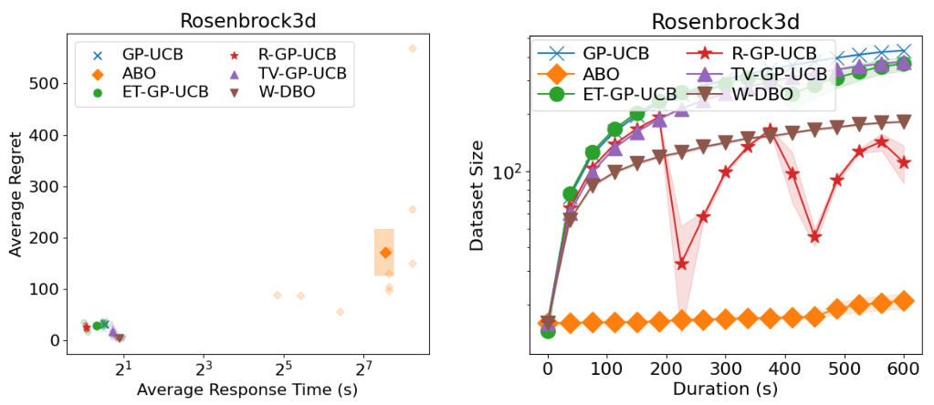
🔼 This figure presents a comparison of different dynamic Bayesian Optimization (DBO) algorithms on the Rosenbrock function. The left panel shows a scatter plot of the average regret (y-axis) versus the average response time (x-axis) for each algorithm. The right panel displays the dataset size of each algorithm over the optimization duration (x-axis). The plots reveal trade-offs between algorithm performance and computational cost.
read the caption
Figure 15: (Left) Average response time and average regrets of the DBO solutions during the optimization of the Rosenbrock synthetic function. (Right) Dataset sizes of the DBO solutions during the optimization of the Rosenbrock synthetic function.
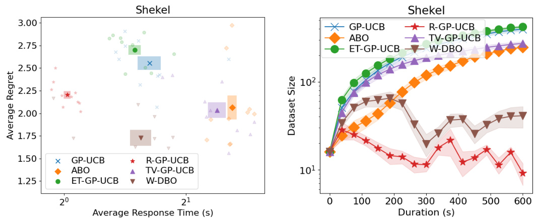
🔼 This figure shows a comparison of different Bayesian Optimization (BO) algorithms on the Shekel synthetic function. The left panel displays average regret (a measure of optimization performance) plotted against average response time. The right panel shows the dataset size of each algorithm over the optimization time. This allows for a comparison of performance, runtime, and dataset management strategies.
read the caption
Figure 16: (Left) Average response time and average regrets of the DBO solutions during the optimization of the Shekel synthetic function. (Right) Dataset sizes of the DBO solutions during the optimization of the Shekel synthetic function.

🔼 This figure compares the performance of different DBO algorithms on the Hartmann-3 benchmark function. The left panel shows average regret (lower is better) plotted against average response time. The right panel shows how the size of the dataset used by each algorithm changes over the duration of the optimization. It provides insights into the trade-off between computational cost and optimization performance for each method, particularly highlighting the impact of observation removal strategies.
read the caption
Figure 17: (Left) Average response time and average regrets of the DBO solutions during the optimization of the Hartmann-3 synthetic function. (Right) Dataset sizes of the DBO solutions during the optimization of the Hartmann-3 synthetic function.
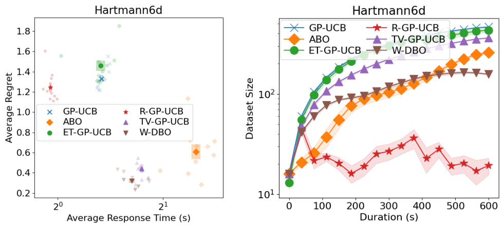
🔼 This figure shows the performance comparison of different dynamic Bayesian optimization (DBO) algorithms on the Hartmann-6 benchmark function. The left panel displays the average regret (a measure of performance) against the average response time of each algorithm. The right panel illustrates the dataset size of each algorithm over the optimization duration. The comparison helps in understanding the trade-off between the accuracy of the model and computational efficiency of different DBO approaches in handling dynamic optimization problems. W-DBO is shown to achieve a good balance.
read the caption
Figure 18: (Left) Average response time and average regrets of the DBO solutions during the optimization of the Hartmann-6 synthetic function. (Right) Dataset sizes of the DBO solutions during the optimization of the Hartmann-6 synthetic function.
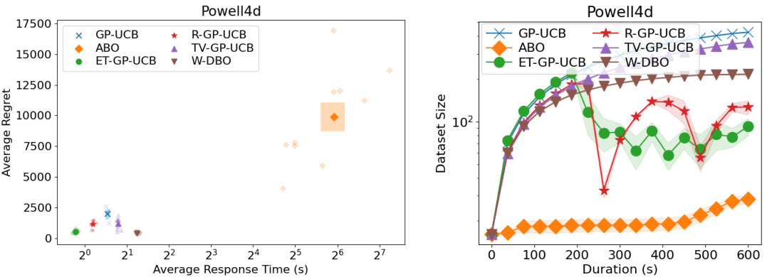
🔼 This figure shows the results of six different DBO algorithms on the Powell synthetic function. The left panel shows the average response time (x-axis) and average regret (y-axis). The right panel shows the dataset sizes used by each algorithm over the duration of the optimization. The results indicate that W-DBO outperforms the other algorithms in terms of both response time and average regret. In addition, W-DBO keeps the dataset size relatively small compared to the other algorithms.
read the caption
Figure 19: (Left) Average response time and average regrets of the DBO solutions during the optimization of the Powell synthetic function. (Right) Dataset sizes of the DBO solutions during the optimization of the Powell synthetic function.
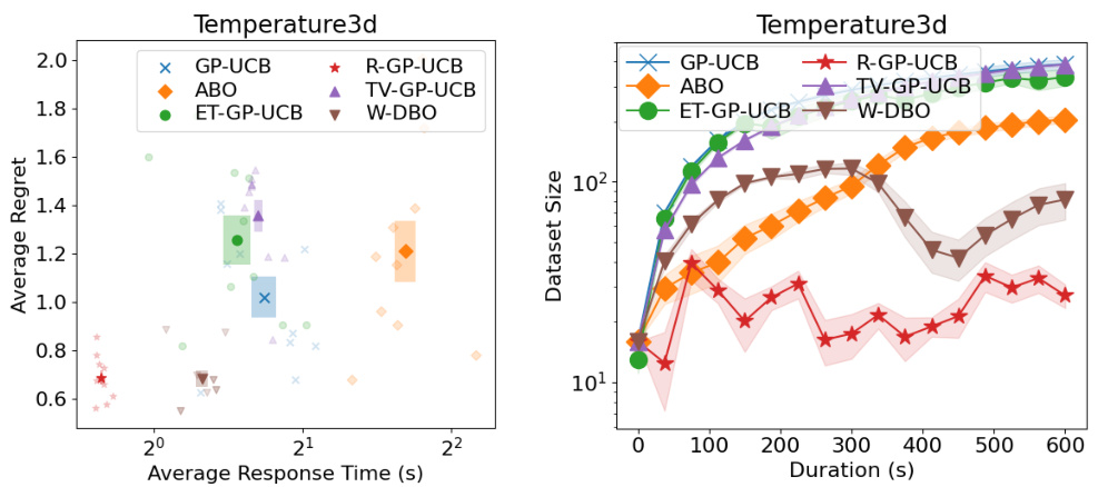
🔼 This figure shows the performance comparison of different DBO algorithms on a real-world temperature dataset. The left panel displays average regret against average response time, illustrating the trade-off between accuracy and efficiency. The right panel shows the dataset size over time for each algorithm, highlighting how different methods manage data over time. The results demonstrate W-DBO’s superior performance in balancing accuracy and dataset size.
read the caption
Figure 20: (Left) Average response time and average regrets of the DBO solutions during the Temperature real-world experiment. (Right) Dataset sizes of the DBO solutions during the Temperature real-world experiment.
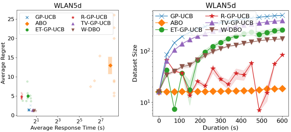
🔼 This figure shows the performance of different DBO algorithms on a real-world WLAN dataset. The left panel displays the average regret (lower is better) plotted against the average response time of each algorithm. The right panel shows the dataset size used by each algorithm over the duration of the experiment. This allows for a comparison of the trade-off between response time (which affects sampling frequency and the ability to track the optimum) and predictive accuracy (which relates to the regret). The plot helps assess the efficiency and effectiveness of each DBO algorithm in balancing these competing factors.
read the caption
Figure 21: (Left) Average response time and average regrets of the DBO solutions during the WLAN real-world experiment. (Right) Dataset sizes of the DBO solutions during the WLAN real-world experiment.
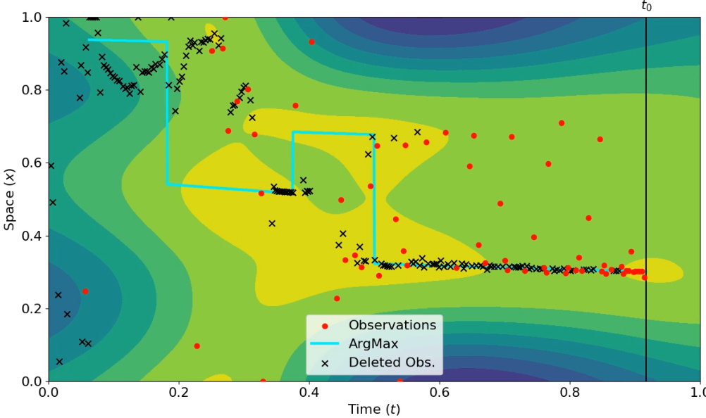
🔼 This figure shows a snapshot of an animation from the paper that illustrates the W-DBO algorithm in action. It displays the algorithm’s performance on a 2D problem where the x-axis represents the normalized time and the y-axis represents the normalized space. Red dots show observations currently used in the model, black crosses show observations that have been deemed irrelevant and discarded, and the cyan line traces the path of the algorithm’s best guess of the optimal solution over time. The contour plot displays the algorithm’s predictions of the objective function. The vertical line labeled ’t0’ indicates the current time.
read the caption
Figure 22: Snapshot from one of the videos showing the optimization conducted by W-DBO. The normalized temporal dimension is shown on the x-axis and the normalized spatial dimension is shown on the y-axis. The observations that are in the dataset are depicted as red dots, while the deleted observations are depicted as black crosses. The maximal arguments \{arg max_{x∈S} f(x,t), t ∈ T\} are depicted with a cyan curve. The predictions of W-DBO are shown with a contour plot. Finally, the present time is depicted as a black vertical line labelled t0.
More on tables

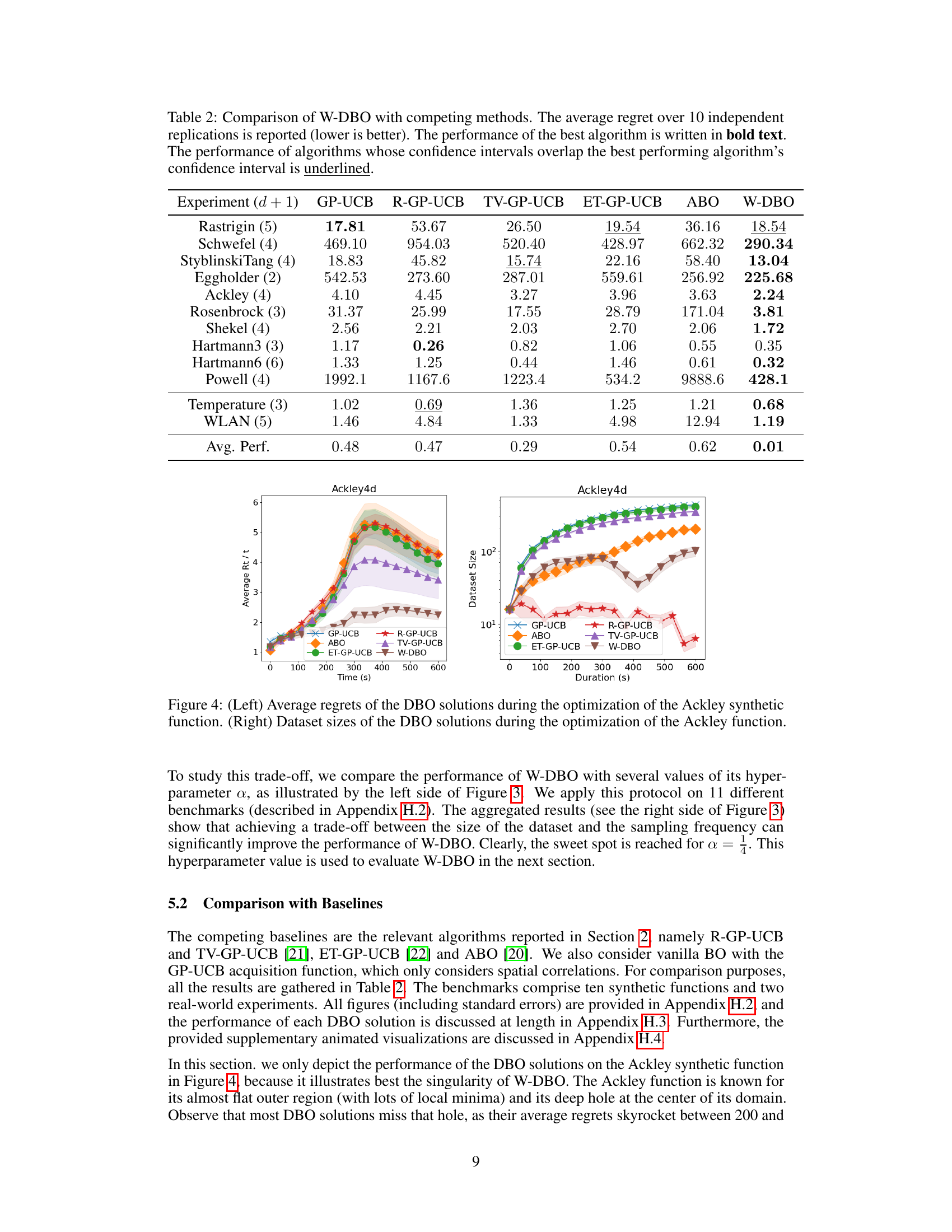
🔼 This table compares the performance of the proposed W-DBO algorithm against several state-of-the-art dynamic Bayesian optimization (DBO) algorithms across various benchmark functions. The average regret, a measure of the algorithm’s cumulative error, is reported for each algorithm. Lower regret values indicate better performance. The best performing algorithm for each benchmark is highlighted in bold. Algorithms with confidence intervals overlapping the best performing algorithm are underlined, indicating statistically similar performance.
read the caption
Table 2: Comparison of W-DBO with competing methods. The average regret over 10 independent replications is reported (lower is better). The performance of the best algorithm is written in bold text. The performance of algorithms whose confidence intervals overlap the best performing algorithm's confidence interval is underlined.

🔼 This table shows the mathematical formulas for two common covariance functions used in Gaussian processes: Squared-Exponential and Matérn. These functions describe the correlation between data points and are parameterized by a length scale (ls) that controls the smoothness and range of the correlation. The Gamma function (Γ) and the modified Bessel function of the second kind (Kv) are special functions used in the formula for the Matérn covariance function.
read the caption
Table 1: Usual covariance functions. Γ is the Gamma function and K, is a modified Bessel function of the second kind of order v.

🔼 This table compares the performance of the W-DBO algorithm to other state-of-the-art dynamic Bayesian Optimization (DBO) algorithms. The comparison is based on the average regret across 10 independent replications for several benchmark functions. Lower average regret indicates better performance. The best performing algorithm for each benchmark is highlighted in bold, and algorithms with confidence intervals overlapping the best performing algorithm are underlined.
read the caption
Table 2: Comparison of W-DBO with competing methods. The average regret over 10 independent replications is reported (lower is better). The performance of the best algorithm is written in bold text. The performance of algorithms whose confidence intervals overlap the best performing algorithm's confidence interval is underlined.

🔼 This table compares two different budget formulas for removing stale observations in the W-DBO algorithm. It shows how the budgets change with different experiment durations (300, 600, and 1800 seconds) and a fixed lengthscale. The comparison highlights the difference in how these formulas scale with time, demonstrating the more consistent behavior of formula (87).
read the caption
Table 5: Comparison of removal budgets (87) and (88) when doing experiments of different durations on the Hartmann3d synthetic function. All experiments use the same time domain [0, 1].
Full paper#
