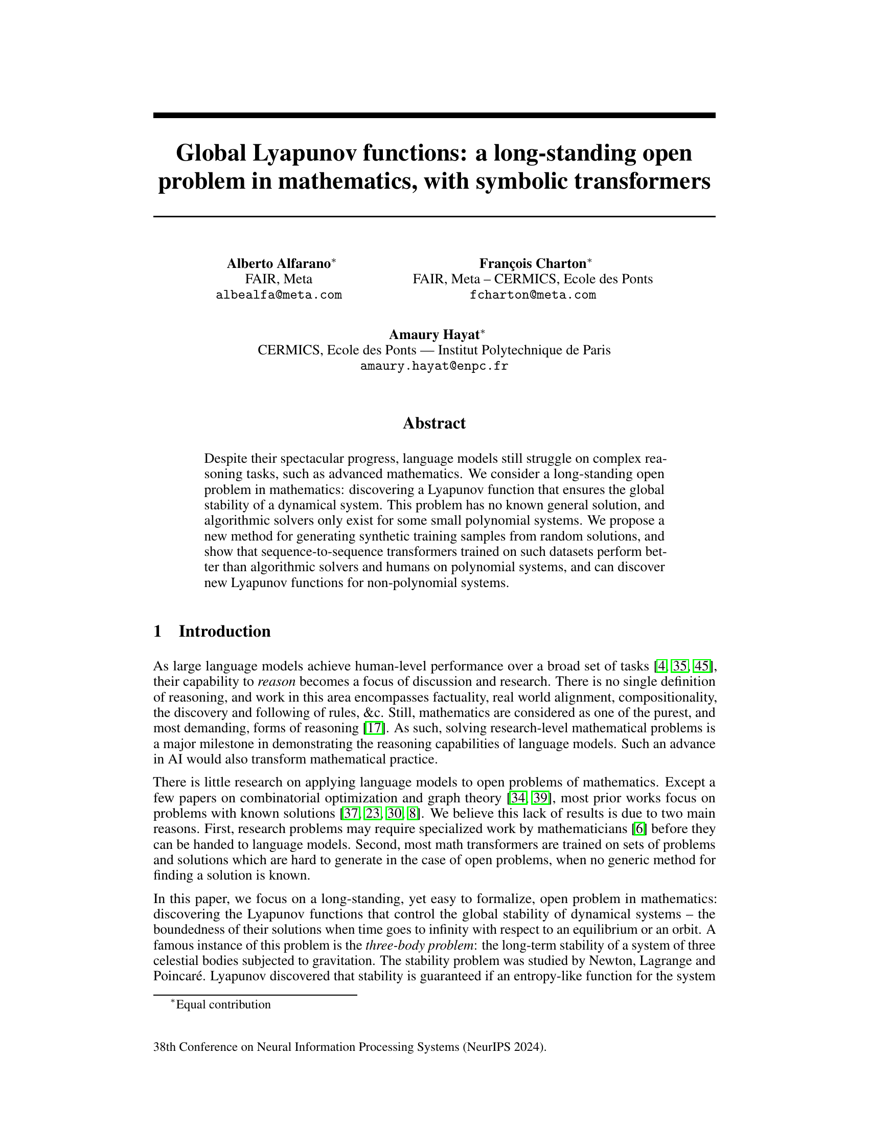
↗ arXiv ↗ Hugging Face ↗ Hugging Face ↗ Chat
TL;DR#
Finding Lyapunov functions to guarantee the stability of dynamical systems is a major unsolved problem in mathematics, crucial for understanding many physical phenomena. Current methods are limited to small, simple systems, hindering progress in diverse fields. The lack of efficient ways to generate training data for AI models further complicates the task.
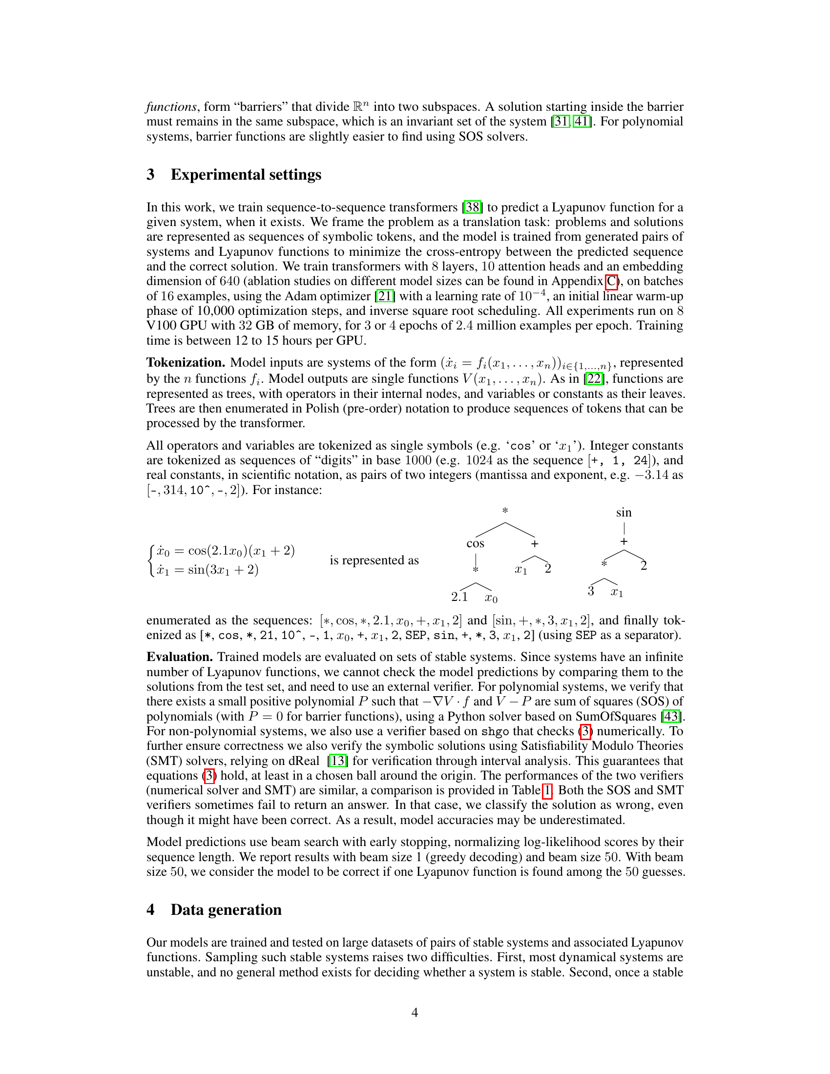
This work introduces a novel approach using sequence-to-sequence transformers. By generating synthetic training data from random Lyapunov functions, the model achieves near-perfect accuracy on known systems. Remarkably, it also discovers new Lyapunov functions for more complex, previously intractable systems. This demonstrates the potential of AI in solving long-standing mathematical challenges and opens new avenues for research in various fields requiring stability analysis.
Key Takeaways#
Why does it matter?#
This paper is crucial because it demonstrates the potential of AI in solving complex mathematical problems that have resisted solution for decades. It bridges the gap between AI and mathematical research, offering a novel method applicable to various fields. The approach’s success opens new avenues for AI-driven discoveries and could revolutionize mathematical practice.
Visual Insights#
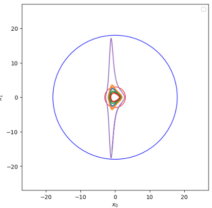
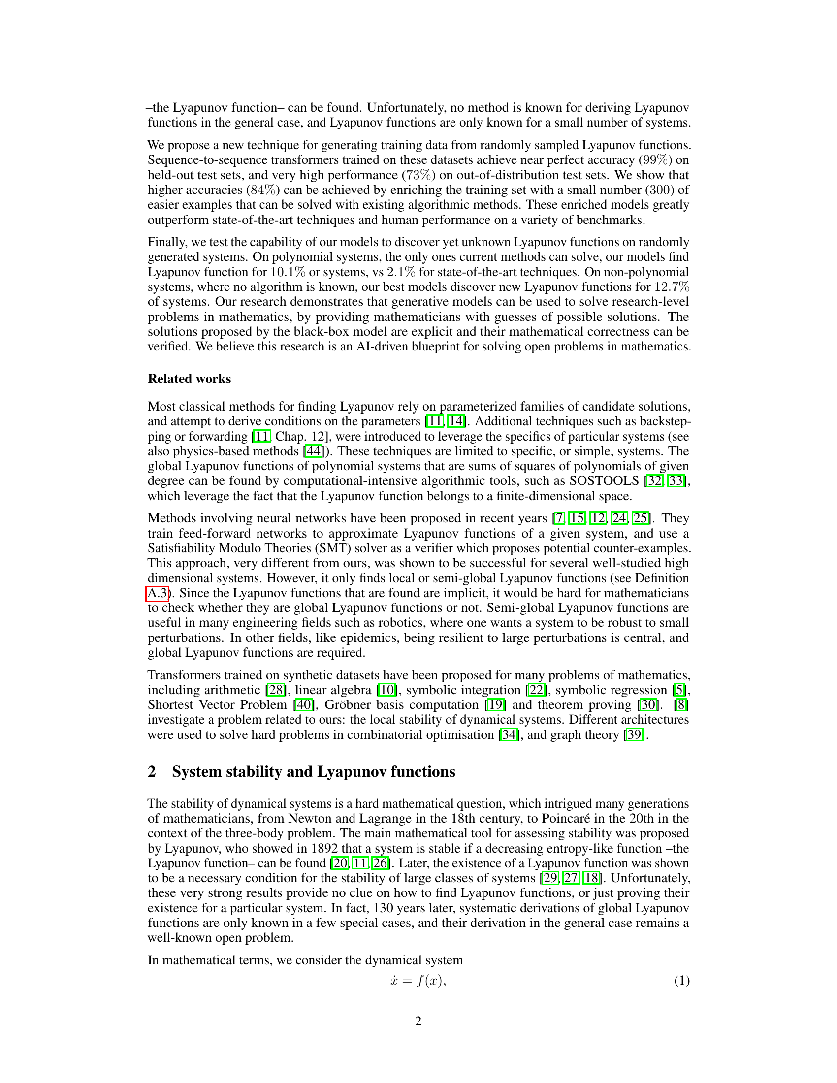
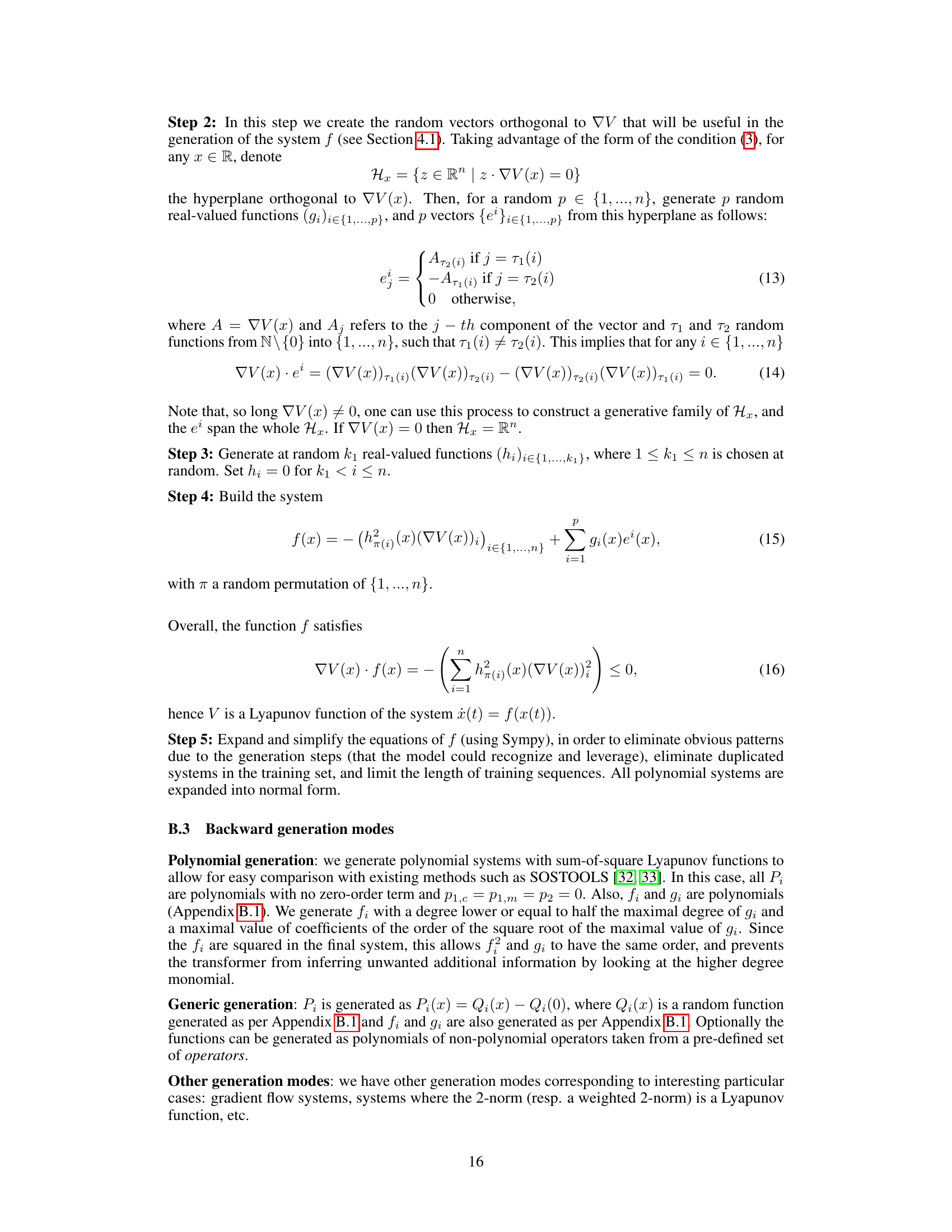
🔼 This figure shows a phase portrait of a stable dynamical system. The trajectories (paths of the system over time) are shown as curves. While the individual trajectories might appear complex and winding, the key point is that all trajectories starting within a certain region (the smaller red circle) remain confined within a larger region (the larger blue circle) as time progresses. This visual illustrates the concept of stability, as the system’s state doesn’t stray too far from the equilibrium point, even if its behavior isn’t immediately obvious from the trajectory shapes.
read the caption
Figure 1: Dynamic of a stable system: trajectories may be complicated but as long as they start in the red ball they remain in the blue ball.

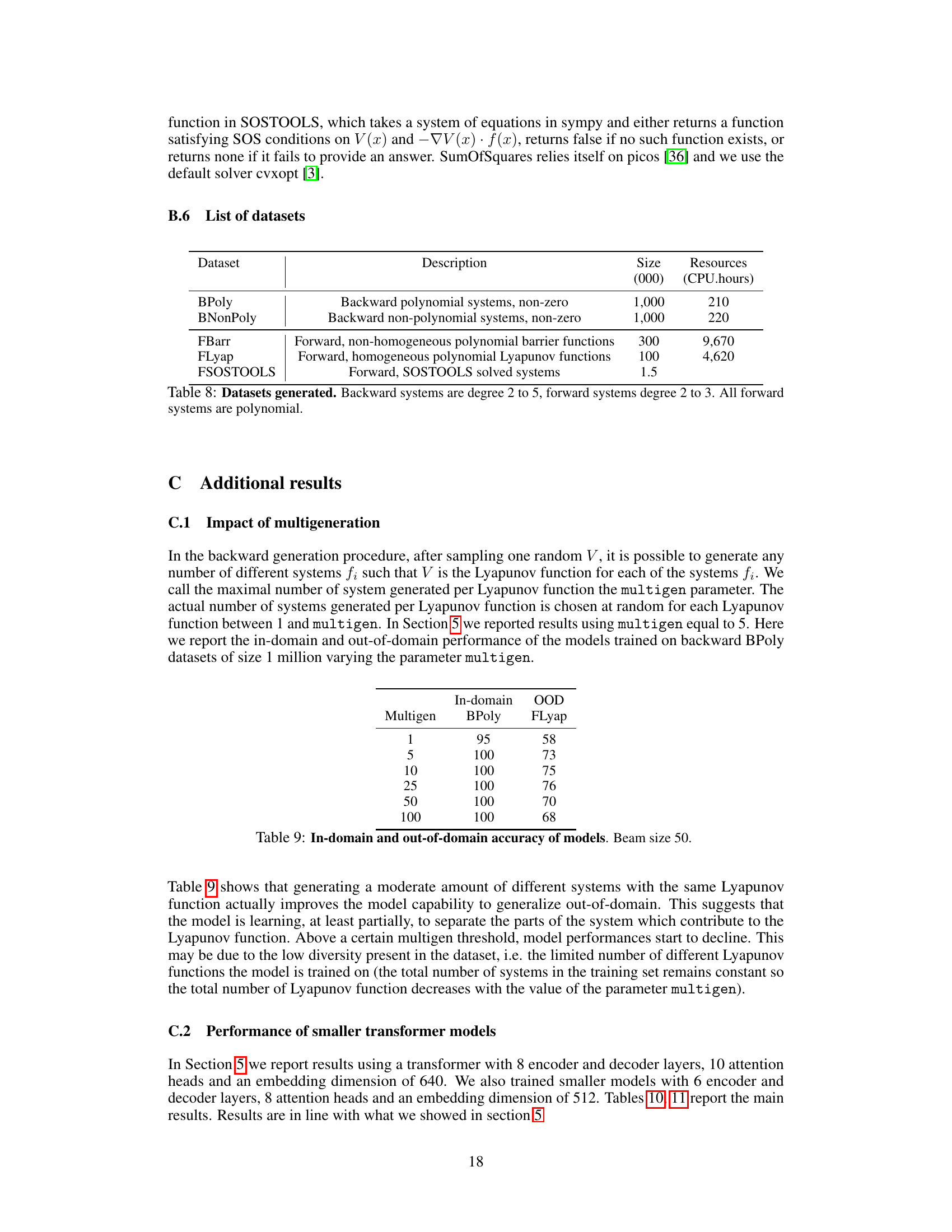
🔼 This table presents the performance of SMT and SOS solvers in verifying the correctness of Lyapunov functions. It shows the percentage of correct Lyapunov functions identified within 10 and 60 minute time limits, as well as the percentage of solver timeouts and incorrect Lyapunov function identifications. The results highlight the trade-off between time constraints and accuracy in verifying Lyapunov functions using these solvers.
read the caption
Table 1: SMT and SOS timeout and error rates, benchmarked on correct Lyapunov functions.
In-depth insights#
Lyapunov Function Search#
The search for Lyapunov functions is a significant challenge in dynamical systems analysis, as they are crucial for establishing stability. This paper tackles this problem by creatively leveraging the power of sequence-to-sequence transformer models. Instead of directly solving for Lyapunov functions, the approach focuses on generating synthetic training data comprised of systems and their corresponding functions. This clever strategy allows the model to learn patterns relating system dynamics to their stability properties, enabling it to predict Lyapunov functions for new, unseen systems. The results demonstrate that transformers, trained on these data, surpass existing algorithmic solvers and even human performance on polynomial systems. More impressively, the model successfully discovers new Lyapunov functions for non-polynomial systems, a domain where traditional methods struggle. This research signifies a major breakthrough, offering a powerful new tool for exploring complex dynamical systems and potentially revolutionizing how stability is analyzed.
Transformer Networks#
Transformer networks, with their self-attention mechanisms, have revolutionized natural language processing. Their ability to process sequential data in parallel, unlike recurrent networks, allows for greater efficiency and scalability. Self-attention enables the model to weigh the importance of different words in a sequence relative to each other, capturing long-range dependencies crucial for understanding context and meaning. This contrasts with recurrent networks which process sequentially, potentially losing information from earlier parts of the sequence. The application of transformers to mathematical problems is a significant development, leveraging their ability to handle symbolic representations and complex reasoning tasks. This offers a powerful new approach to solving problems with no known algorithmic solution by learning patterns from data. While the ‘black box’ nature of deep learning models might limit interpretability, the demonstrable effectiveness of these methods highlights their potential for significant advancements in tackling challenging mathematical problems. The key to successful application lies in crafting appropriate training data, allowing the model to learn the intricate relationships inherent in mathematical structures and processes.
Synthetic Data Gen#
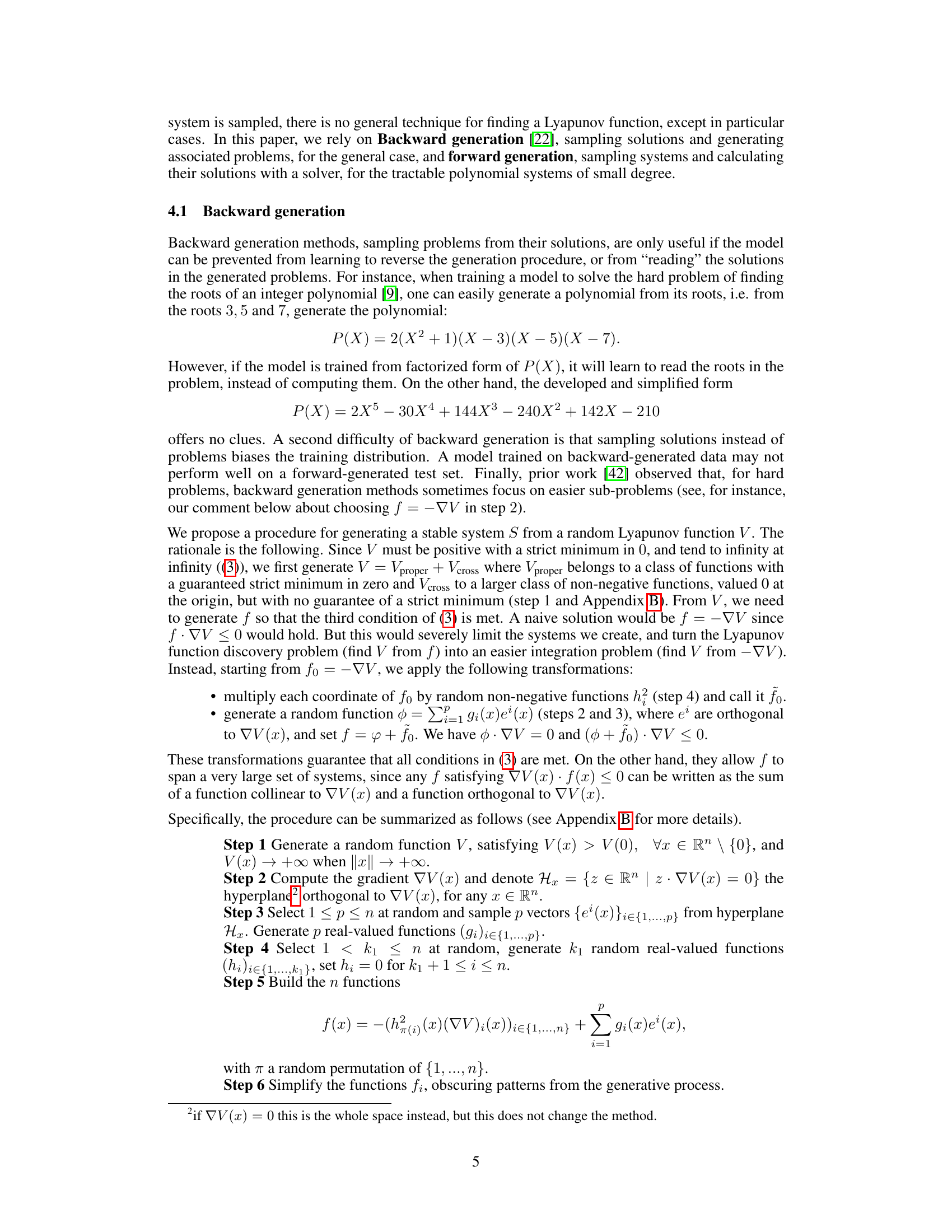
Synthetic data generation for training machine learning models is a crucial aspect of many research papers. In the context of a research paper focusing on Lyapunov functions, synthetic data generation would likely involve creating pairs of dynamical systems and their corresponding Lyapunov functions. The complexity arises from the inherent difficulty in finding Lyapunov functions for arbitrary systems. A successful strategy might employ a two-pronged approach: first generating stable systems using methods that guarantee stability, and second, constructing Lyapunov functions for those systems using established mathematical techniques or by sampling from known families of such functions. The quality of the synthetic data is paramount. It must accurately reflect the complexity and characteristics of real-world data to ensure the trained model generalizes well. This includes considerations of data distribution, noise levels, and the representation of both the systems and functions, likely as symbolic sequences. Careful design of the data generation process is essential to avoid biases and to create a sufficiently diverse and representative dataset, improving the model’s ability to learn the intricate relationships between systems and Lyapunov functions.
Limitations of Methods#
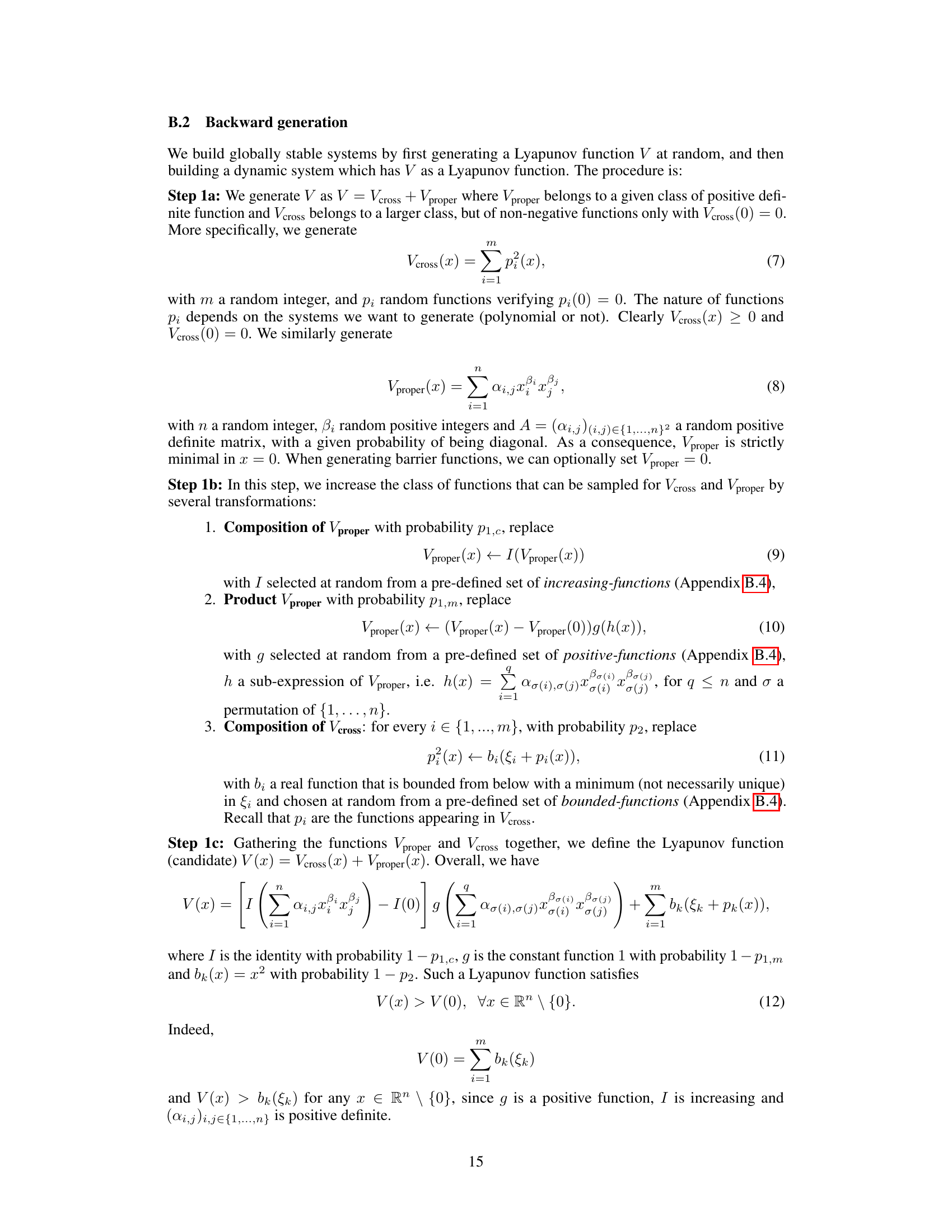
The core limitation lies in the reliance on synthetic data generation. Backward generation, while ingenious, might inadvertently bias the model towards easily solvable problems, hindering generalization to truly novel, complex systems. Furthermore, the forward generation method, employing existing SOS solvers, suffers from computational constraints, limiting dataset size and the diversity of solvable polynomial systems. The study acknowledges these limitations, but further research could explore more robust data augmentation techniques, potentially incorporating real-world data or employing alternative stability verification methods to circumvent reliance on SOS solvers. Generalization to higher-dimensional systems or non-polynomial dynamics remains a significant challenge, necessitating future work to assess the model’s performance in those domains. The paper’s reliance on specific verifiers also limits general applicability; future work should consider alternative verification methods. While the model demonstrates impressive capabilities, its success relies heavily on the quality and diversity of the training dataset, highlighting the importance of addressing dataset limitations to further enhance the model’s robustness and predictive accuracy.
Future Research#
Future research directions stemming from this work on discovering Lyapunov functions using symbolic transformers are multifaceted. Extending the approach to higher-dimensional systems is crucial, as current methods struggle with scaling. This requires exploring more efficient data generation techniques and potentially adapting the transformer architecture for improved performance in higher-dimensional spaces. Investigating the applicability of this method to other open problems in mathematics is another promising avenue. The success in solving this long-standing problem suggests that generative models combined with symbolic reasoning can unlock solutions for other complex mathematical challenges. Further research into the theoretical underpinnings of why this approach is successful is vital. Understanding the connection between the structure of Lyapunov functions, the generated training data, and the architecture of the transformer would provide valuable insights. A detailed comparison with other AI-based methods designed for solving similar problems is needed to better assess the strengths and weaknesses of the proposed technique. The development of robust verification methods for non-polynomial systems would also significantly enhance the impact of this work. Addressing these research questions will further solidify the use of AI in mathematical discovery and open new possibilities for solving complex scientific challenges.
More visual insights#
More on tables

🔼 This table presents the in-domain accuracy results of the trained models. In-domain accuracy refers to how well the models perform on data from the same dataset they were trained on. The table shows the accuracy for two beam sizes (1 and 50), with beam size 50 allowing the model to provide multiple possible solutions. Two backward datasets (BPoly and BNonPoly) and two forward datasets (FBarr and Flyap) are included, showcasing performance differences across different model types and data sources.
read the caption
Table 2: In-domain accuracy of models. Beam size (bs) 1 and 50.

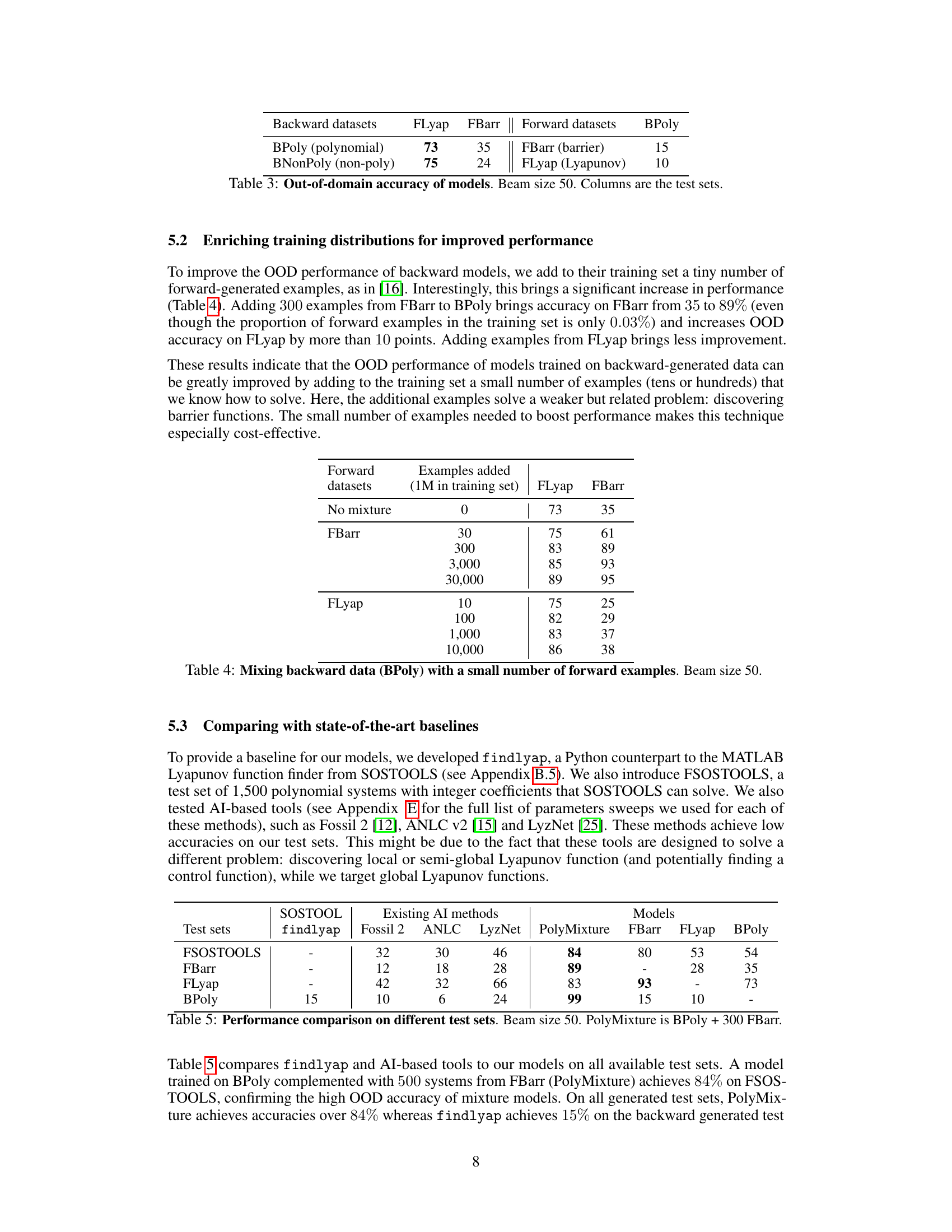
🔼 This table presents the out-of-distribution accuracy results of the models trained on the backward datasets when tested on the forward datasets and vice versa. It demonstrates the models’ ability to generalize beyond the datasets used for training. The lower accuracy on some cross-dataset tests highlights challenges in generalizing across differing distributions of Lyapunov functions and system types.
read the caption
Table 3: Out-of-domain accuracy of models. Beam size 50. Columns are the test sets.

🔼 This table presents the results of experiments where a small number of forward-generated examples are added to the backward-generated training data (BPoly). It shows how the addition of examples from either the FBarr (barrier functions) or FLyap (Lyapunov functions) datasets affects the model’s accuracy on the held-out test sets (FLyap and FBarr). The beam size used for the model was 50.
read the caption
Table 4: Mixing backward data (BPoly) with a small number of forward examples. Beam size 50.

🔼 This table compares the performance of different methods for discovering Lyapunov functions on various test sets. It shows the accuracy of SOSTOOLS, findlyap (a Python implementation of SOSTOOLS), three AI-based methods (Fossil 2, ANLC, LyzNet), and the authors’ models (PolyMixture, FBarr, FLyap, BPoly). The test sets represent different types of systems (polynomial and non-polynomial) and Lyapunov functions (general and barrier functions). PolyMixture represents a model enhanced with additional training data.
read the caption
Table 5: Performance comparison on different test sets. Beam size 50. PolyMixture is BPoly + 300 FBarr.

🔼 This table presents the percentage of correct solutions found by different models on three datasets of random systems: polynomial systems with 2 or 3 equations (Poly3), polynomial systems with 2 to 5 equations (Poly5), and non-polynomial systems with 2 or 3 equations (NonPoly). It compares the performance of SOSTOOLS, other AI methods (Fossil 2, ANLC, LyzNet), and the authors’ models (FBarr, PolyM, NonPolyM). The results demonstrate that the authors’ models trained on generated datasets can discover unknown Lyapunov functions.
read the caption
Table 6: Discovering Lyapunov comparison for random systems. Beam size 50. PolyM is BPoly + 300 FBarr. NonPolyM is BNonPoly + BPoly + 300 FBarr.

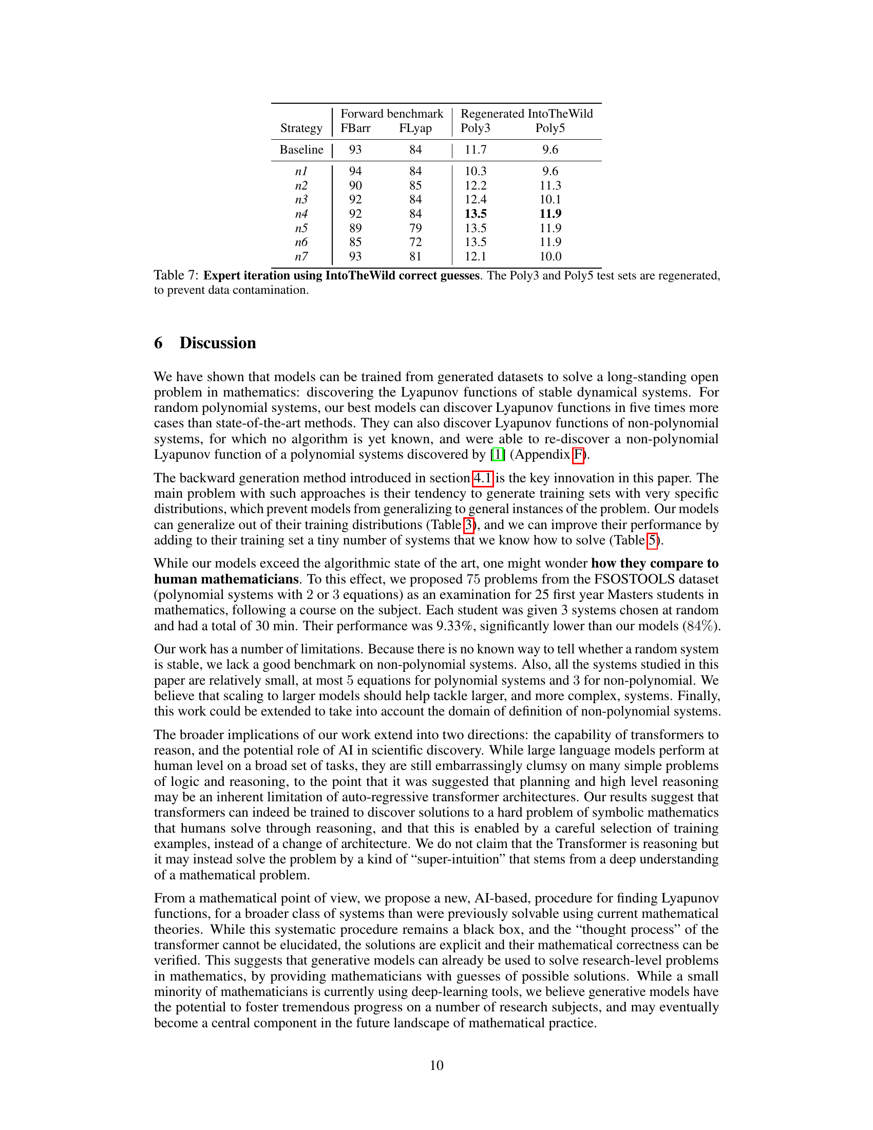
🔼 This table presents the results of an expert iteration process, where newly solved problems (from the FIntoTheWild set) are added to the model’s training data. It shows the performance (accuracy) of different strategies, comparing in-domain (FBarr, FLyap) and out-of-distribution (Poly3, Poly5) results after fine-tuning. The strategies vary in the number and type of additional examples added. The goal is to evaluate the impact of incorporating real-world problem solutions on the model’s ability to solve similar problems.
read the caption
Table 7: Expert iteration using IntoTheWild correct guesses. The Poly3 and Poly5 test sets are regenerated, to prevent data contamination.

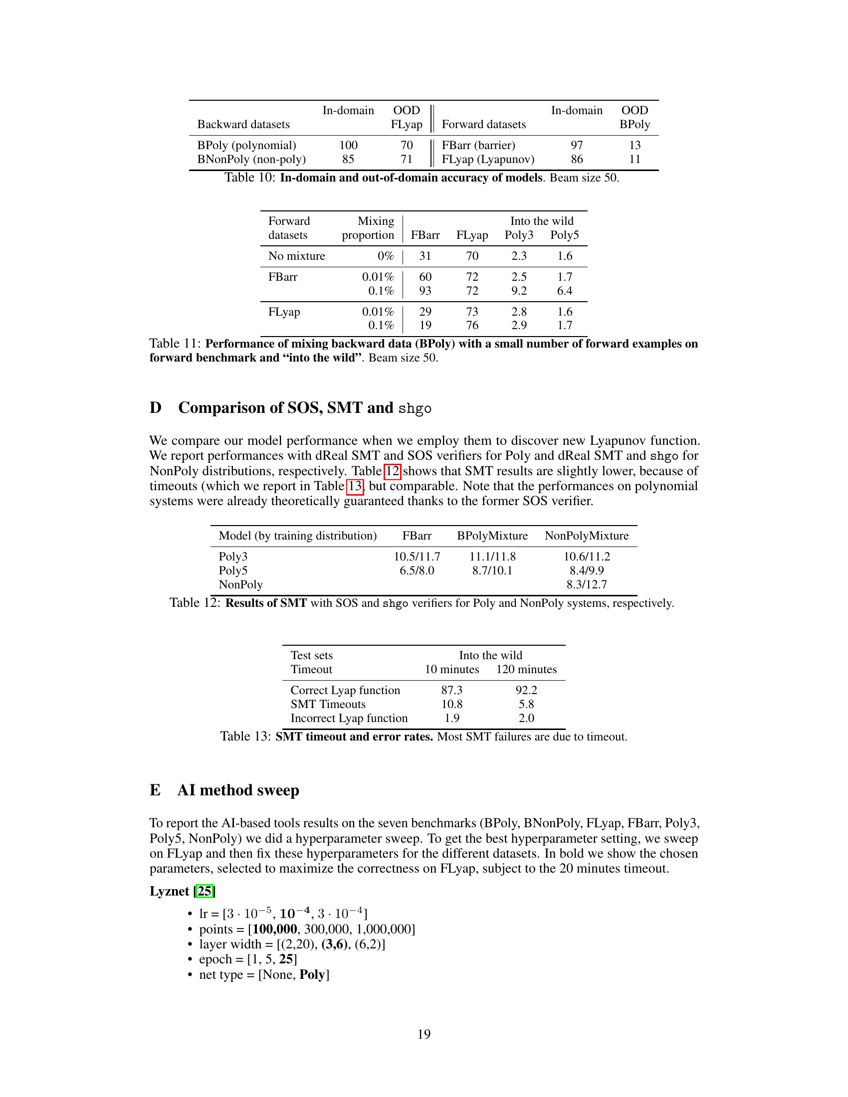
🔼 This table lists the five datasets used in the paper’s experiments. It shows the dataset name, a description of the dataset contents (whether it contains backward-generated or forward-generated samples, and whether the Lyapunov functions are polynomial or not), the size of the dataset in thousands of samples, and the approximate CPU hours required for generation.
read the caption
Table 8: Datasets generated. Backward systems are degree 2 to 5, forward systems degree 2 to 3. All forward systems are polynomial.

🔼 This table presents the in-domain and out-of-domain accuracy of models trained on the backward BPoly dataset of size 1 million, varying the multigen parameter. The multigen parameter controls the number of different systems generated per Lyapunov function. The table shows that generating a moderate amount of different systems with the same Lyapunov function improves the model’s ability to generalize out-of-domain. However, above a certain threshold, the performance starts to decrease.
read the caption
Table 9: In-domain and out-of-domain accuracy of models. Beam size 50.

🔼 This table shows the out-of-distribution (OOD) accuracy of models trained on different datasets. The rows represent the training datasets (backward datasets: BPoly, BNonPoly; forward datasets: FBarr, FLyap), and the columns represent the test datasets. The high accuracy of backward models on forward test sets and vice versa demonstrates their ability to generalize across different data distributions. The lower accuracy of forward models on backward datasets suggests that the forward training data is less diverse.
read the caption
Table 3: Out-of-domain accuracy of models. Beam size 50. Columns are the test sets.
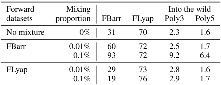
🔼 This table shows the impact of adding a small number of forward examples to the training data of backward models. It demonstrates how adding just 300 examples from the FBarr dataset to the BPoly training data significantly boosts performance on the FBarr and FLyap datasets. The results are shown for both the forward benchmark and out-of-distribution 'into the wild' tests, demonstrating improved generalization.
read the caption
Table 11: Performance of mixing backward data (BPoly) with a small number of forward examples on forward benchmark and \'into the wild\' . Beam size 50.

🔼 This table presents the percentage of correct solutions found by different models on three datasets of random systems: polynomial systems with 2 or 3 equations (Poly3), polynomial systems with 2 to 5 equations (Poly5), and non-polynomial systems with 2 or 3 equations (NonPoly). It compares the performance of SOSTOOLS, other AI-based methods, and two transformer-based models (FBarr and PolyM/NonPolyM) in discovering Lyapunov functions for these randomly generated systems. The results show that the transformer-based models significantly outperform the other methods, especially on the non-polynomial dataset.
read the caption
Table 6: Discovering Lyapunov comparison for random systems. Beam size 50. PolyM is BPoly + 300 FBarr. NonPolyM is BNonPoly + BPoly + 300 FBarr.

🔼 This table presents the performance of SMT and SOS solvers in verifying the correctness of Lyapunov functions. It shows the percentage of correct Lyapunov functions, the percentage of timeouts, and the percentage of incorrect Lyapunov functions identified by the solvers. The results are broken down based on the time allocated to each solver (10 and 60 minutes). The table provides insights into the reliability and efficiency of the different solvers in evaluating Lyapunov functions.
read the caption
Table 1: SMT and SOS timeout and error rates, benchmarked on correct Lyapunov functions.
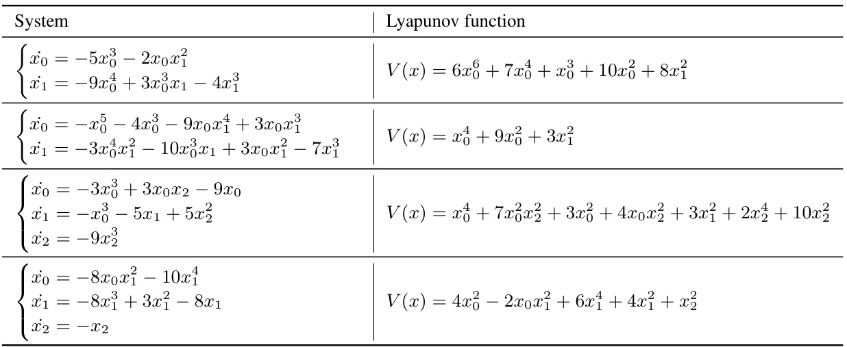
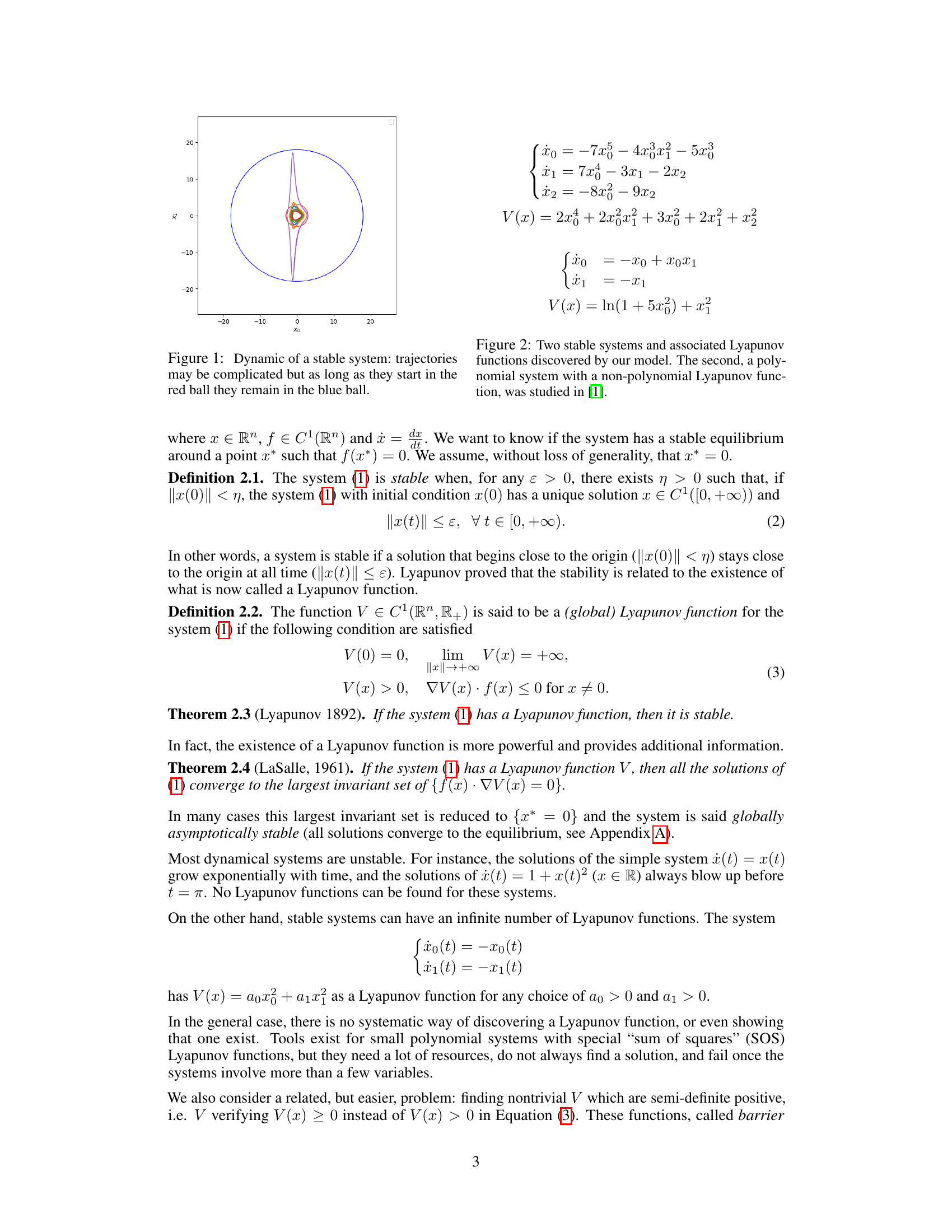
🔼 This table presents four examples of systems (left column) and their corresponding Lyapunov functions (right column) discovered by the model. Each system is a set of differential equations, and the Lyapunov function is a scalar function that helps demonstrate the stability of the system.
read the caption
Table 14: Some additional examples generated from our models.
Full paper#
