TL;DR#
Multi-Output Regression (MOR) faces challenges with high-dimensional outputs, hindering interpretability and scalability. Existing methods often lack efficiency or fail to consider the inherent sparsity in many real-world applications. This necessitates novel approaches that can balance predictive accuracy with computational feasibility and enhanced interpretability.
This research introduces SHORE, a Sparse & High-dimensional-Output Regression model, which incorporates sparsity requirements. A two-stage optimization framework efficiently solves SHORE via output compression. Theoretically, the framework ensures computational scalability and maintains accuracy. Empirical results validate the framework’s efficiency and accuracy on both synthetic and real-world datasets, showcasing its potential for diverse applications.
Key Takeaways#
Why does it matter?#
This paper is important because it offers a computationally efficient and accurate framework for handling high-dimensional output regression problems, a common challenge in modern machine learning. The SHORE model and its associated algorithm are valuable for researchers working with large datasets and complex output structures. The theoretical guarantees and empirical results presented provide a strong foundation for future research in this area, especially concerning high-dimensional data analysis, algorithmic trading, and model interpretability.
Visual Insights#

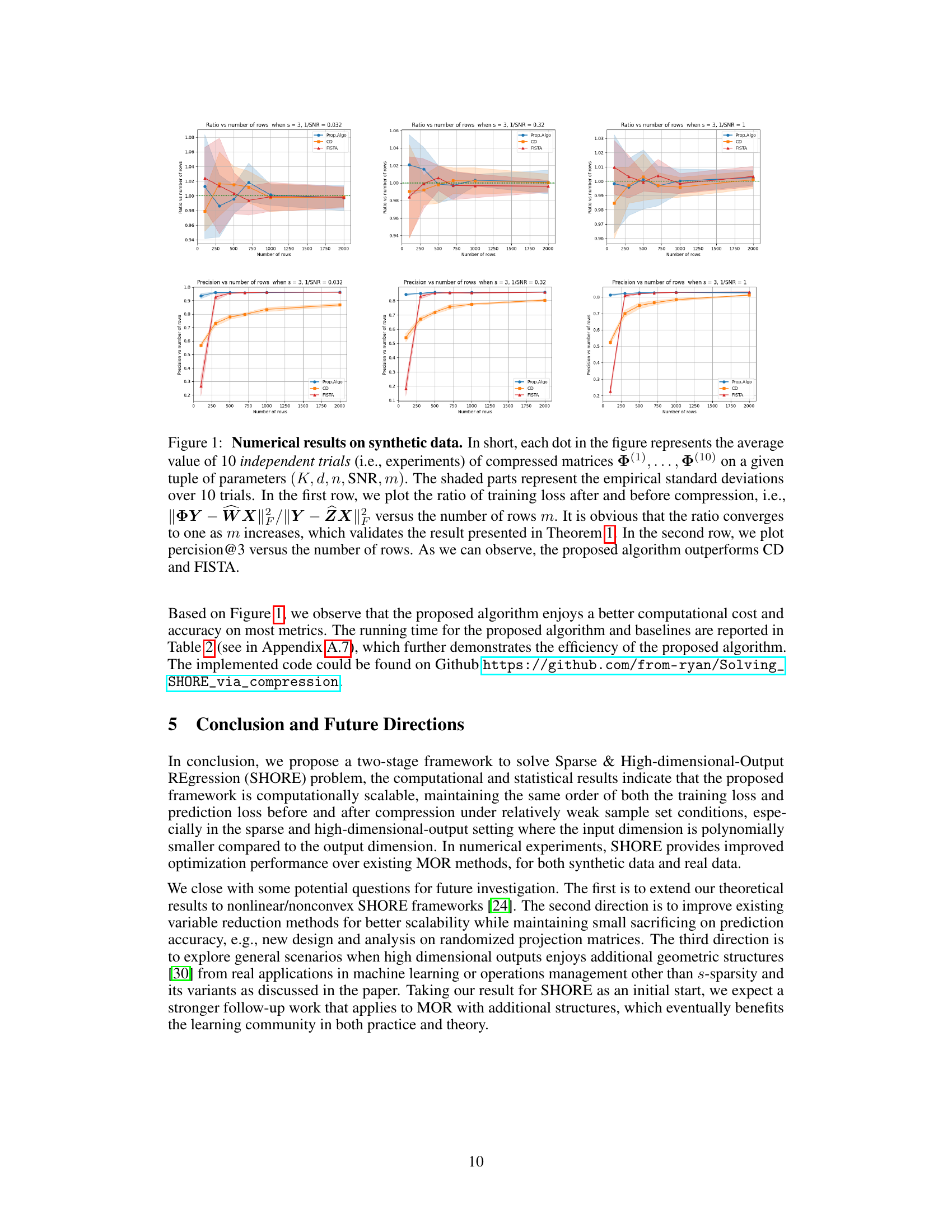
🔼 The figure shows numerical results on synthetic data to validate the theoretical findings and illustrate the efficiency and accuracy of the proposed algorithm. The first row presents the ratio of training loss after and before compression versus the number of rows (m), demonstrating convergence to one as m increases. The second row shows precision@3 (the percentage of correctly identified supports in the predicted output) versus m, indicating the superiority of the proposed algorithm over other methods.
read the caption
Figure 1: Numerical results on synthetic data. In short, each dot in the figure represents the average value of 10 independent trials (i.e., experiments) of compressed matrices Φ(1), ..., Φ(10) on a given tuple of parameters (K, d, n, SNR, m). The shaded parts represent the empirical standard deviations over 10 trials. In the first row, we plot the ratio of training loss after and before compression, i.e., ||ΦY – WX|||||Y – ZX|| versus the number of rows m. It is obvious that the ratio converges to one as m increases, which validates the result presented in Theorem 1. In the second row, we plot percision@3 versus the number of rows. As we can observe, the proposed algorithm outperforms CD and FISTA.

🔼 This table presents the statistics of the training and test sets used in the numerical experiments of the paper. It shows the input dimension (d), output dimension (K), and the number of samples (n) for both the training and test sets for two datasets: EURLex-4K and Wiki10-31K. Additionally, the average number of non-zero components for both input (d) and output (K) are provided for each set. This information is crucial for understanding the scale and characteristics of the data used in evaluating the proposed model and comparing it with existing baselines.
read the caption
Table 1: Statistics and details for training and test sets, where d, K denote their averaged non-zero components for input and output, respectively.
In-depth insights#
MOR Interpretability#
Multi-output regression (MOR) models, while powerful for predicting multiple outputs, often suffer from interpretability challenges. The high dimensionality of outputs makes understanding the model’s decision-making process difficult. Sparsity constraints can enhance interpretability by focusing on a smaller subset of relevant outputs. However, introducing sparsity adds complexity to the model and optimization process. Compression techniques, such as dimensionality reduction applied to the output space, offer a potential solution by creating a lower-dimensional representation which maintains important information while simplifying the model and improving computational efficiency. Further research might focus on developing more sophisticated compression methods tailored for MOR that preserve output interpretability and achieve accurate predictions, while addressing the trade-off between sparsity and accuracy in a principled way. Methods that incorporate domain knowledge into the selection of outputs could further boost interpretability by aligning the relevant outputs with the problem context.
SHORE Framework#
The SHORE (Sparse & High-dimensional-Output REgression) framework tackles the challenges of interpretability and scalability in multi-output regression problems, particularly those with high-dimensional sparse outputs. Its core innovation lies in a two-stage approach: First, it compresses the high-dimensional output space into a lower-dimensional latent space using a compression matrix. This compression significantly reduces computational complexity during training, making the method scalable for large datasets. The second stage leverages a computationally efficient iterative algorithm (projected gradient descent) to reconstruct a sparse output vector in the original high-dimensional space. This two-stage approach enables SHORE to balance interpretability (via sparsity constraints) and computational efficiency. Theoretical analysis provides guarantees on the training and prediction loss after compression, showing that SHORE maintains accuracy while significantly reducing the computational burden. The effectiveness and efficiency of the SHORE framework are further demonstrated empirically with experiments on both synthetic and real-world datasets, showcasing its advantages over traditional multi-output regression methods.
Compression Analysis#
A compression analysis in a research paper would typically involve a detailed examination of the techniques used to reduce data size, and their impact on performance and model accuracy. This could include discussions of various compression algorithms (lossy or lossless), dimensionality reduction methods, and the trade-offs between compression ratio and information loss. A key aspect would be the quantitative evaluation of the compressed data’s performance compared to the original, uncompressed data, using metrics relevant to the task (e.g., accuracy, precision, recall for classification; MSE, RMSE for regression). The analysis should explore how different compression parameters (e.g., compression ratio, quantization levels) affect the results and identify the optimal balance between data size and performance. Furthermore, a comprehensive analysis would likely involve considerations of computational cost, memory usage, and implementation complexity associated with the chosen compression methods. Theoretical analysis, including mathematical proofs or bounds, may also be included to support the empirical findings and explain the performance behavior under various conditions. Ultimately, a thorough compression analysis strives to provide a clear understanding of the strengths and limitations of different compression strategies within the specific context of the research problem, aiding in the selection of the most effective and efficient approach.
Empirical Validation#
An empirical validation section in a research paper is crucial for establishing the credibility and practical significance of the presented methodology. It involves conducting experiments using real-world or simulated data and comparing the results against established baselines or theoretical predictions. A strong validation should clearly define the metrics used, providing both quantitative and qualitative analyses. It’s essential to demonstrate the proposed approach’s performance across various datasets and parameters, highlighting its robustness and generalizability. A thoughtful discussion of results, addressing limitations and potential biases is paramount, thus allowing researchers to assess the extent to which the study’s findings generalize to other scenarios. The inclusion of error bars or confidence intervals is vital for demonstrating statistical significance and reliability, while visualizations such as graphs and tables can effectively present results and facilitate a clearer understanding of the findings. Reproducibility is key, hence the section needs to meticulously document the experimental setup, including data sources, software versions, and parameter choices. A comprehensive empirical validation provides compelling evidence to support the research claims, adding a layer of trustworthiness and impact to the overall work.
Future Extensions#
The research paper’s ‘Future Extensions’ section would ideally explore several key avenues. Extending the framework to handle non-linear relationships between inputs and outputs is crucial for broader applicability. The current linear model, while computationally efficient, may limit accuracy in real-world scenarios. Investigating non-convex loss functions, beyond the squared error, could improve robustness to outliers and better capture complex data distributions. Developing adaptive compression strategies that dynamically adjust the dimensionality reduction based on the input data’s characteristics would further optimize performance and interpretability. This would involve intelligent selection of the compression matrix Φ, perhaps via a learned approach. A deeper examination of the generalization error bounds under weaker distributional assumptions is also warranted. The current light-tailed distribution assumption might be overly restrictive. Finally, applying the methodology to diverse, real-world datasets from different domains (beyond finance and algorithmic trading) is essential to fully validate its practicality and scalability, potentially uncovering unforeseen challenges or opportunities for improvement. These extensions would significantly broaden the scope and impact of the research.
More visual insights#
More on figures
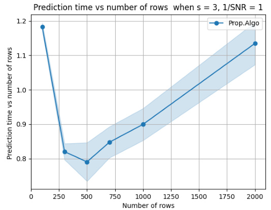
🔼 The figure displays numerical results obtained from synthetic data to validate the proposed algorithm’s performance. It shows four sets of graphs. The first row shows the ratio of training loss before and after compression plotted against the number of rows (m) in the compressed matrix. This demonstrates the relationship between compression and training loss, supporting Theorem 1. The second row displays precision@3 (a measure of the algorithm’s accuracy) against the number of rows (m). This comparison highlights the superiority of the proposed algorithm over existing methods (CD and FISTA).
read the caption
Figure 1: Numerical results on synthetic data. In short, each dot in the figure represents the average value of 10 independent trials (i.e., experiments) of compressed matrices Φ(1), ..., Φ(10) on a given tuple of parameters (K, d, n, SNR, m). The shaded parts represent the empirical standard deviations over 10 trials. In the first row, we plot the ratio of training loss after and before compression, i.e., ||ΦY – WX|||||Y – ZX|| versus the number of rows m. It is obvious that the ratio converges to one as m increases, which validates the result presented in Theorem 1. In the second row, we plot percision@3 versus the number of rows. As we can observe, the proposed algorithm outperforms CD and FISTA.
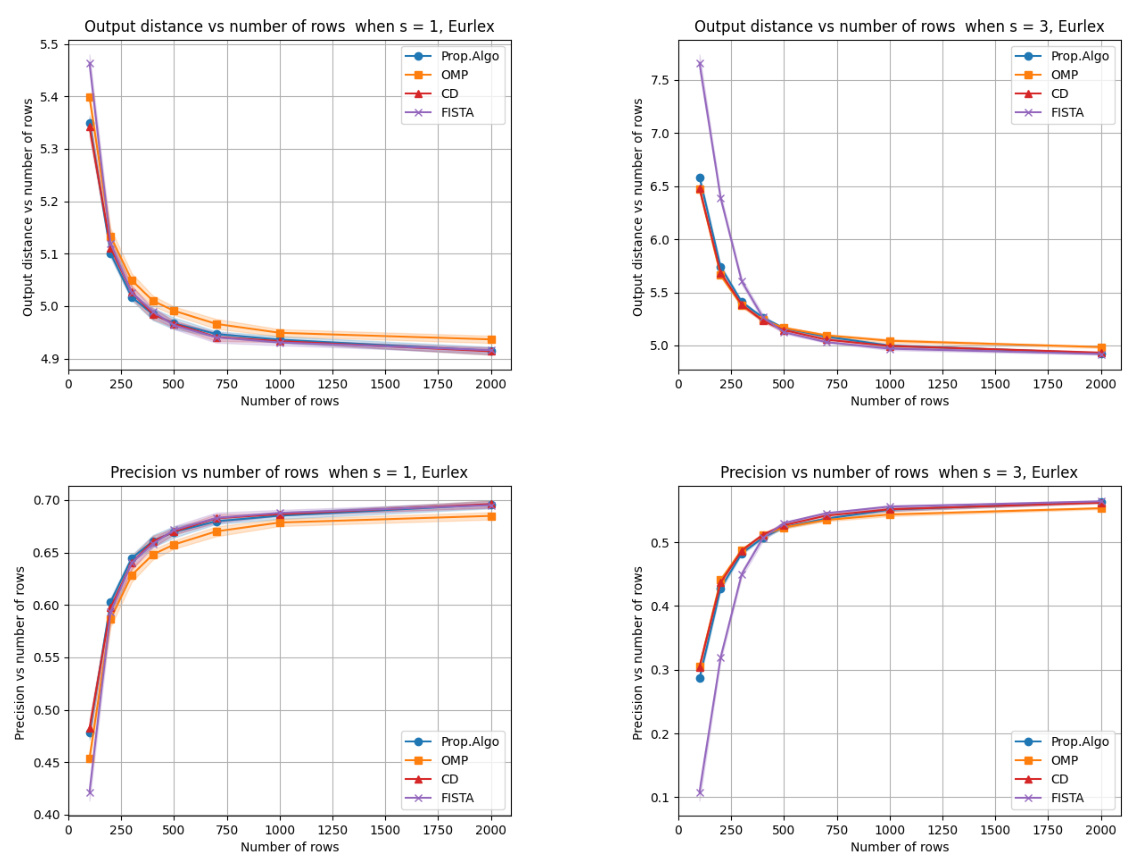
🔼 This figure presents the results of numerical experiments on the EURLex-4K dataset, comparing the proposed algorithm to baselines (OMP, CD, FISTA) for different sparsity levels (s=1 and s=3). The top row shows the output distance (a measure of prediction accuracy) against the number of rows (m) in the compressed matrix. The bottom row shows precision (a measure of the number of correctly identified features) against the number of rows (m). The results illustrate the performance of the proposed algorithm relative to the baselines. The shaded area represents the standard deviation over 10 trials, suggesting the stability of the algorithm’s performance. While there are minor differences, the differences between the algorithms are relatively small.
read the caption
Figure 3: This figure reports the numerical results on real data – EURLex-4K. Each dot in the figure represents 10 independent trials (i.e., experiments) of compressed matrices Φ(1),...,Φ(10) on a given tuple of parameters (s,m). The curves in each panel correspond to the averaged values for the proposed Algorithm and baselines over 10 trials; the shaded parts represent the empirical standard deviations over 10 trials. In the first row, we plot the output distance versus the number of rows. In the second row, we plot the precision versus the number of rows, and we cannot observe significant differences between these prediction methods.

🔼 The figure presents numerical results obtained from experiments on synthetic data. The experiments assess the performance of the proposed algorithm and its comparison with other baseline algorithms by varying several parameters, including the number of rows (m), signal-to-noise ratio (SNR), and sparsity level (s). The plots show the ratio of training loss before and after compression and the precision@3 metric. The results indicate that the ratio of training losses converges to 1 as m increases, verifying Theorem 1. The precision@3 metric demonstrates the proposed algorithm’s superior performance compared to other baselines.
read the caption
Figure 1: Numerical results on synthetic data. In short, each dot in the figure represents the average value of 10 independent trials (i.e., experiments) of compressed matrices Φ(1), ..., Φ(10) on a given tuple of parameters (K, d, n, SNR, m). The shaded parts represent the empirical standard deviations over 10 trials. In the first row, we plot the ratio of training loss after and before compression, i.e., ||ΦY – WX|||||Y – ZX|| versus the number of rows m. It is obvious that the ratio converges to one as m increases, which validates the result presented in Theorem 1. In the second row, we plot percision@3 versus the number of rows. As we can observe, the proposed algorithm outperforms CD and FISTA.
Full paper#


