TL;DR#
Many machine learning tasks require sampling from probability distributions, especially in Bayesian inference. However, sampling from constrained domains (where the data must lie within a specific region) presents a significant challenge. Existing methods, such as those based on Markov Chain Monte Carlo (MCMC) or variational inference (VI), often struggle with constrained domains, either being computationally expensive or lacking accuracy. They often rely on specific assumptions or intricate techniques tailored to particular types of constraints, limiting their widespread applicability.
This paper introduces a novel method called Constrained Functional Gradient Flow (CFG) to address this challenge. CFG utilizes a functional gradient flow framework with a key boundary condition to ensure particles stay within the constrained region. This approach provides a general solution applicable to domains with various shapes and constraints. The authors provide theoretical analysis demonstrating the method’s convergence and further support their claims with extensive experimental results across multiple constrained machine learning tasks. CFG proves to be superior to existing state-of-the-art methods in both efficiency and accuracy.
Key Takeaways#
Why does it matter?#
This paper is crucial because it presents a novel approach to constrained sampling, a persistent challenge in various fields. The proposed method, CFG, offers a general solution applicable to various constrained domains, demonstrating significant improvements over existing techniques. This opens up exciting possibilities for improved Bayesian inference, machine learning models, and other applications needing efficient sampling in complex spaces. The theoretical guarantees and experimental results support the effectiveness and efficiency of the proposed framework, paving the way for broader adoption in research.
Visual Insights#
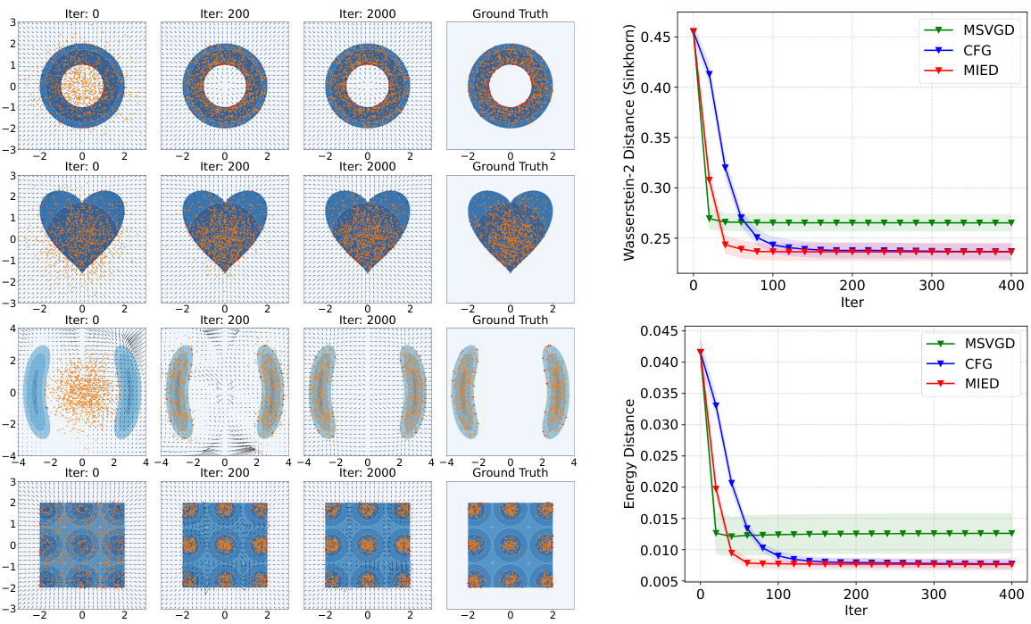
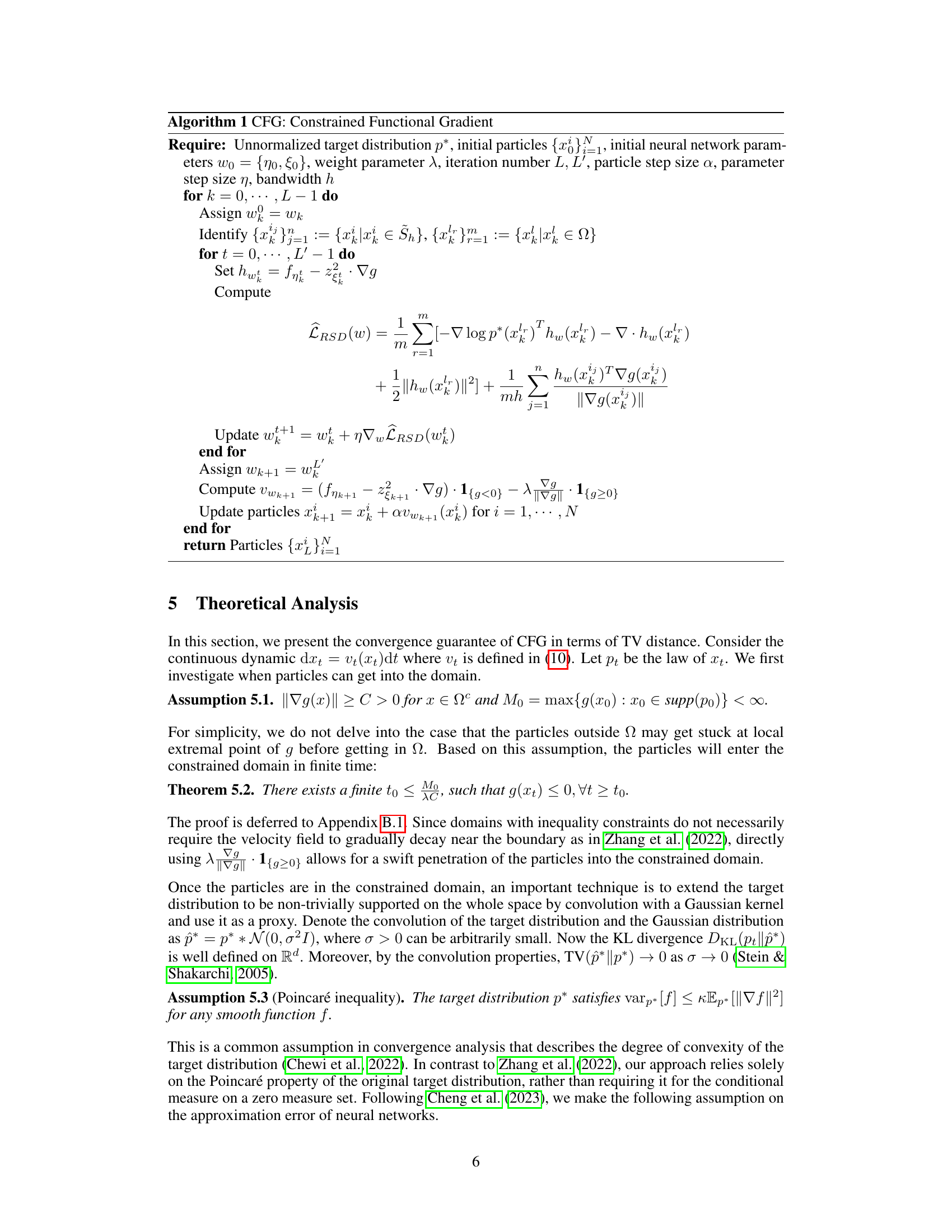
🔼 This figure demonstrates the effectiveness of the proposed CFG method on sampling from four different truncated Gaussian distributions within various constrained domains. The left panel shows the particle distributions at different iterations for each of the four domains: ring, cardioid, double-moon, and block. The particles successfully converge to their respective target distributions without escaping the constrained domains. The right panel displays the convergence curves of MSVGD, CFG, and MIED methods for the block constraint. These curves are plotted using Wasserstein-2 distance and energy distance metrics against the number of iterations and illustrate that CFG demonstrates superior convergence performance compared to the baseline methods, MIED and MSVGD.
read the caption
Figure 1: Left: CFG sampled particles at different numbers of iterations on constrained domains (ring, cardioid, double-moon, block). Right: The convergence curves of MSVGD, CFG and MIED on the block constraint.

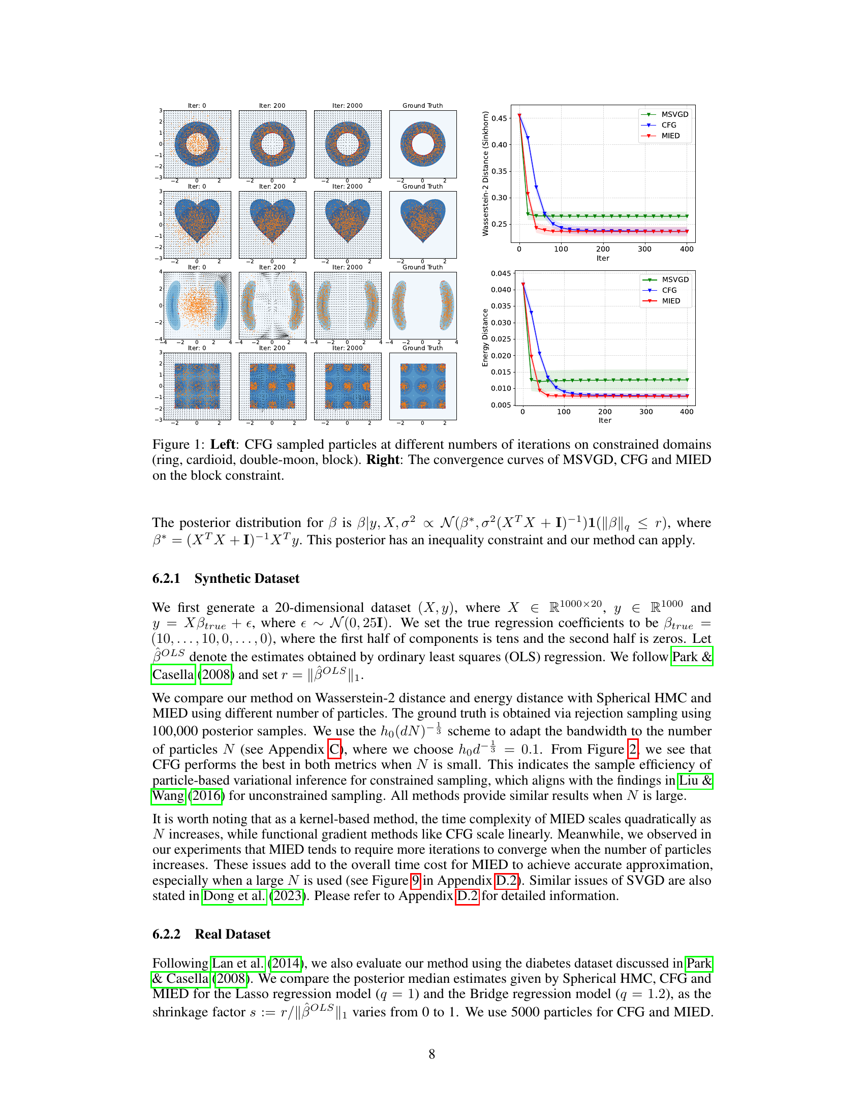
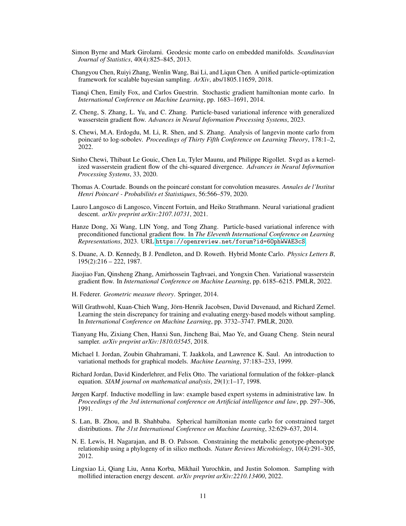
🔼 This table presents the results of a monotonic Bayesian neural network experiment under various monotonicity thresholds (0.05, 0.01, and 0.005). The table shows the test accuracy (TEST ACC), test negative log-likelihood (TEST NLL), and the ratio of particles outside the constrained domain (RATIO OUT (%)). The results for each metric are presented for four different methods: PD-SVGD, C-SVGD, MIED, and the proposed CFG method. The average results are taken from the last 10 checkpoints to enhance robustness.
read the caption
Table 1: Results of monotonic Bayesian neural network under different monotonicity threshold. The results are averaged from the last 10 checkpoints for robustness.
In-depth insights#
Constrained ParVI#
Constrained ParVI methods address the challenge of sampling from probability distributions confined to specific domains. Traditional particle-based variational inference (ParVI) techniques often struggle in constrained spaces, as particles may escape the designated region. Constrained ParVI modifies ParVI algorithms by incorporating boundary conditions into the gradient flow. This ensures particles remain within the domain during the iterative sampling process. Several approaches exist, such as imposing constraints through penalty functions, using projection methods to keep particles within boundaries or designing particle update rules that explicitly respect the constraints. The choice of method depends on the complexity of the constraints and the desired balance between computational cost and accuracy. A key challenge is effectively handling the boundary conditions, which often requires sophisticated numerical techniques. Furthermore, theoretical guarantees regarding the convergence and accuracy of constrained ParVI methods are crucial for ensuring reliable results and are an active area of research. The effectiveness of these methods hinges on the ability to accurately represent the constrained distribution and the computational efficiency of the boundary handling. Future research directions include exploring more general constraint types and developing more robust theoretical analysis for improved performance and reliability.
Boundary Handling#
Effective boundary handling is crucial for sampling algorithms operating within constrained domains. Ignoring boundaries can lead to inaccurate samples and biased results, as particles may escape the desired region. The paper tackles this by introducing a boundary condition into the gradient flow, ensuring particles remain within the constraints. This approach is more general than methods relying on specific geometric transformations, enabling application to diverse and complex constraints. However, imposing boundary conditions necessitates handling boundary integrals, which are often intractable. The paper proposes novel numerical strategies to approximate these integrals effectively, thus avoiding computationally expensive numerical techniques. The success of these approximation methods will be highly dependent on selecting appropriate bandwidth parameters, impacting both accuracy and efficiency. Theoretical analysis demonstrates convergence properties in total variation, providing a solid foundation for the method’s reliability. Ultimately, the effectiveness of this boundary handling strategy hinges on the balance between accuracy, computational cost, and the complexities of handling general boundary shapes.
CFG Convergence#
The convergence analysis of the Constrained Functional Gradient Flow (CFG) method is a crucial aspect of the research paper. It aims to provide theoretical guarantees for the proposed algorithm’s ability to effectively sample from probability distributions within constrained domains. The analysis likely involves establishing bounds on the total variation (TV) distance between the empirical particle distribution generated by CFG and the true target distribution. A key element would be proving that the TV distance decreases over time, converging to zero under specific conditions. Assumptions about the target distribution (e.g., smoothness, log-concavity, Poincaré inequality) are likely to be made to ensure the convergence proof’s tractability. The convergence rate (how fast the TV distance goes to zero) would be another important finding, as it demonstrates the method’s efficiency and practicality. The role of the boundary conditions in the convergence analysis is critical. They are instrumental in ensuring that the particle remain confined within the target domain during the iterative update process. The authors would show how these boundary conditions influence the gradient flow and contribute to convergence. Numerical experiments should demonstrate how the proposed theoretical convergence rate compares to actual convergence behavior, further solidifying the algorithm’s performance and robustness.
Method Extensions#
Method extensions in research papers often involve adapting existing techniques to new domains or problems. A thoughtful approach to evaluating these extensions necessitates examining their novelty, the rationale behind the modifications, and their empirical validation. Novelty might involve addressing limitations of prior work, exploring alternative theoretical frameworks, or applying methods to significantly different problem settings. The rationale for extensions should be clearly articulated and justified. Empirical results are crucial; extensions should be rigorously evaluated to demonstrate their effectiveness compared to existing methods and to pinpoint their strengths and weaknesses. In addition, a critical analysis should assess the generalizability of the extended methods. Do they perform well across various datasets or parameter settings? Finally, the discussion should acknowledge any limitations inherent in the extended approach and provide insights for future research directions. Properly addressing these aspects provides a comprehensive and insightful evaluation of method extensions.
Future Directions#
Future research could explore extending the CFG framework to handle more complex constraints, such as those involving multiple inequality constraints or constraints on manifolds. Investigating the theoretical properties of CFG under weaker assumptions on the target distribution would enhance its applicability. Developing more efficient numerical strategies for approximating the boundary integral is crucial, particularly for high-dimensional problems. Furthermore, a comparison with other constrained sampling methods using a broader range of benchmark datasets and tasks would strengthen the evaluation. Finally, research could focus on applying CFG to more challenging real-world problems within machine learning and beyond, potentially advancing the fields of Bayesian inference and probabilistic modeling.
More visual insights#
More on figures
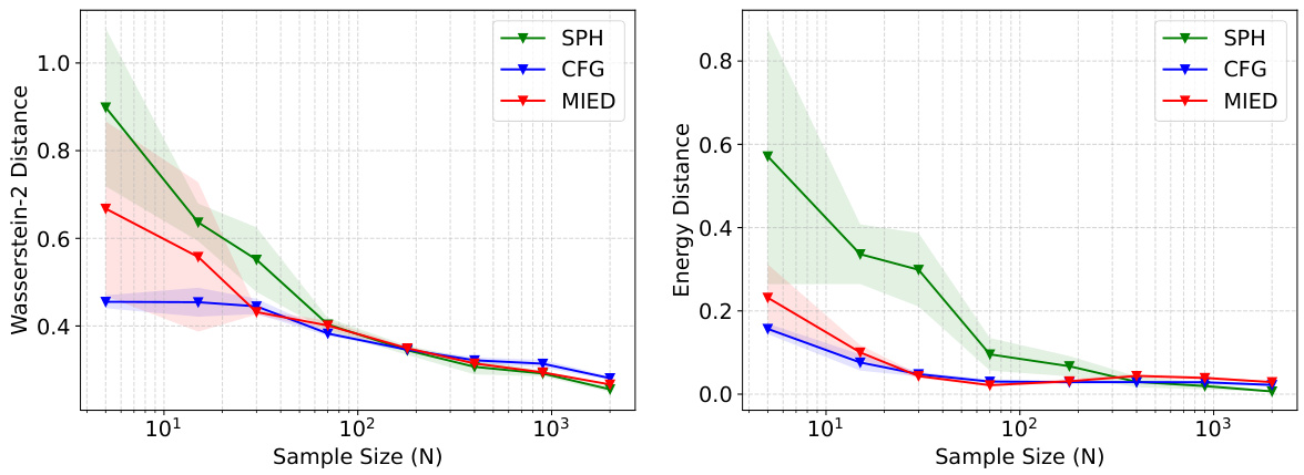
🔼 The left part of the figure shows the effectiveness of the CFG method in sampling from four different truncated Gaussian distributions within various constrained domains. The right part shows the convergence of the CFG, MSVGD, and MIED methods on the block-shaped domain using Wasserstein-2 distance and energy distance as metrics.
read the caption
Figure 1: Left: CFG sampled particles at different numbers of iterations on constrained domains (ring, cardioid, double-moon, block). Right: The convergence curves of MSVGD, CFG and MIED on the block constraint.
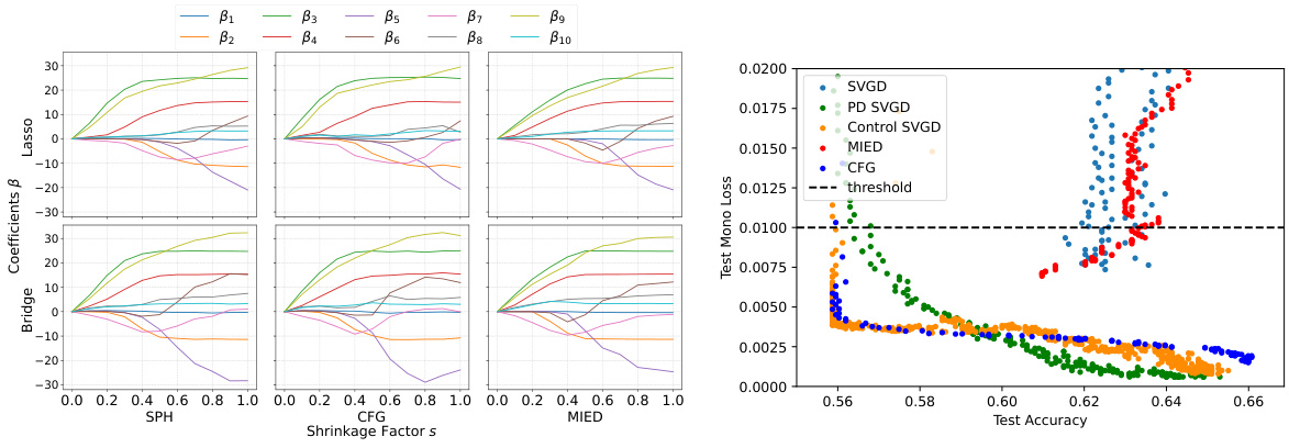
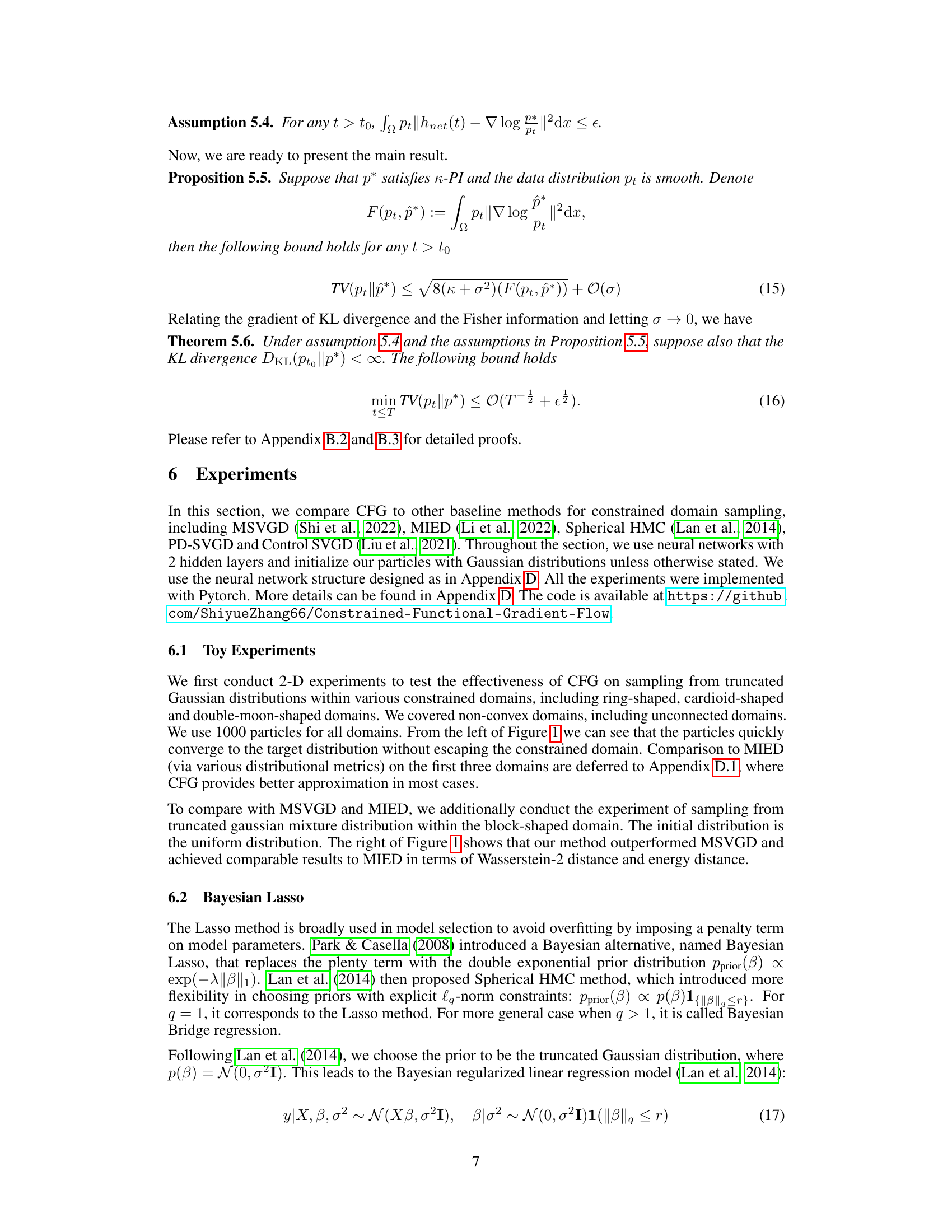
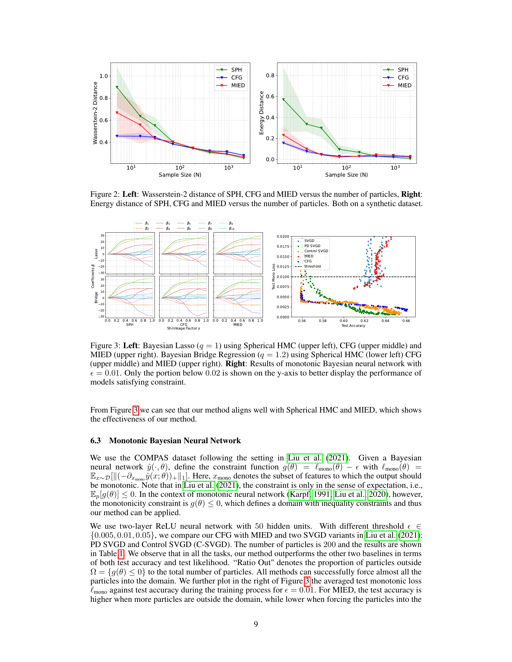
🔼 This figure presents the comparison results of Bayesian Lasso and Bayesian Bridge Regression using three different methods: Spherical HMC, CFG, and MIED. The left part shows the estimated coefficients of the models, and the right part shows the test accuracy and test monotonic loss of a monotonic Bayesian neural network trained with different methods. The results indicate that CFG achieves comparable performance to MIED and better performance than Spherical HMC.
read the caption
Figure 3: Left: Bayesian Lasso (q = 1) using Spherical HMC (upper left), CFG (upper middle) and MIED (upper right). Bayesian Bridge Regression (q = 1.2) using Spherical HMC (lower left) CFG (upper middle) and MIED (upper right). Right: Results of monotonic Bayesian neural network with ε = 0.01. Only the portion below 0.02 is shown on the y-axis to better display the performance of models satisfying constraint.

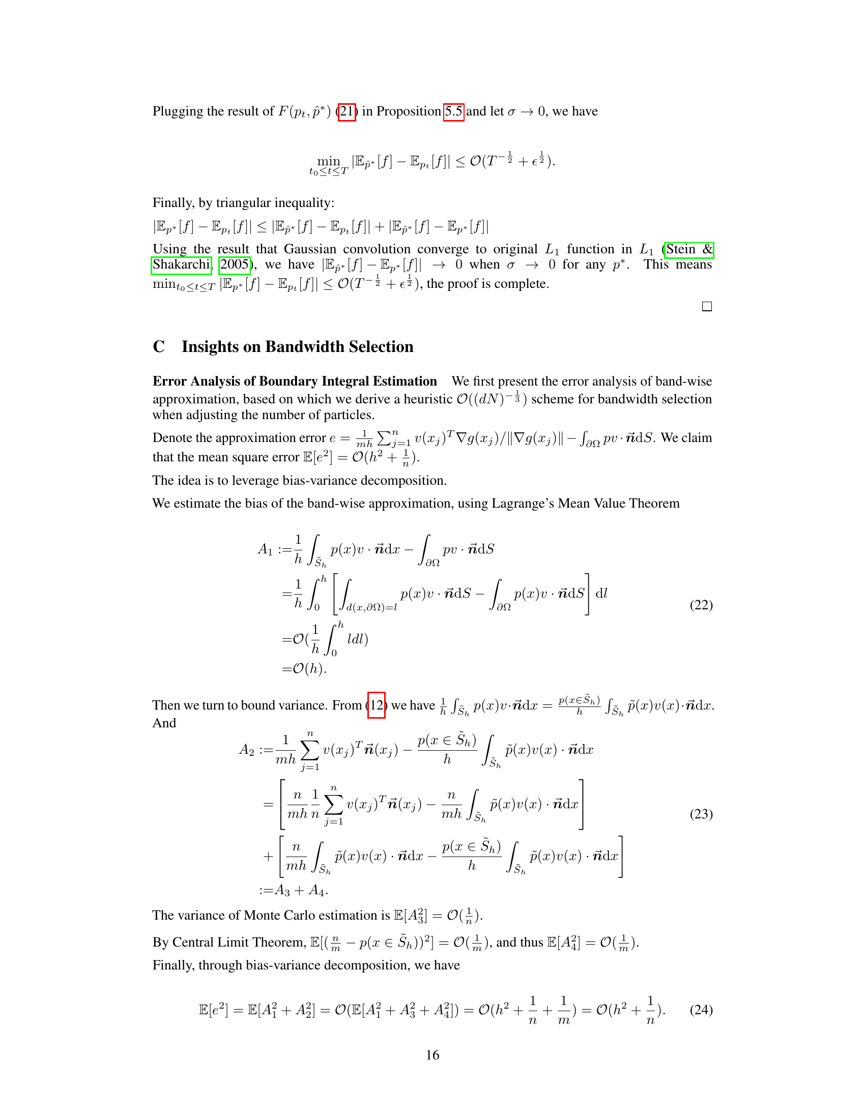
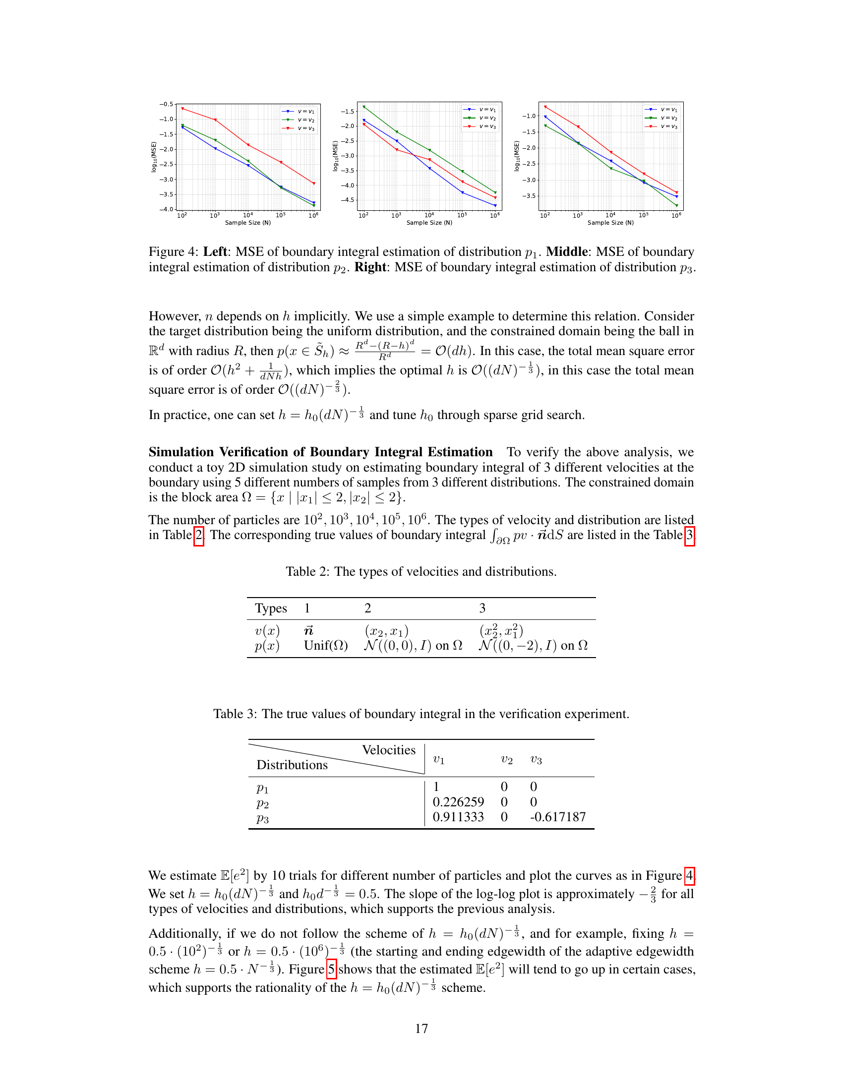
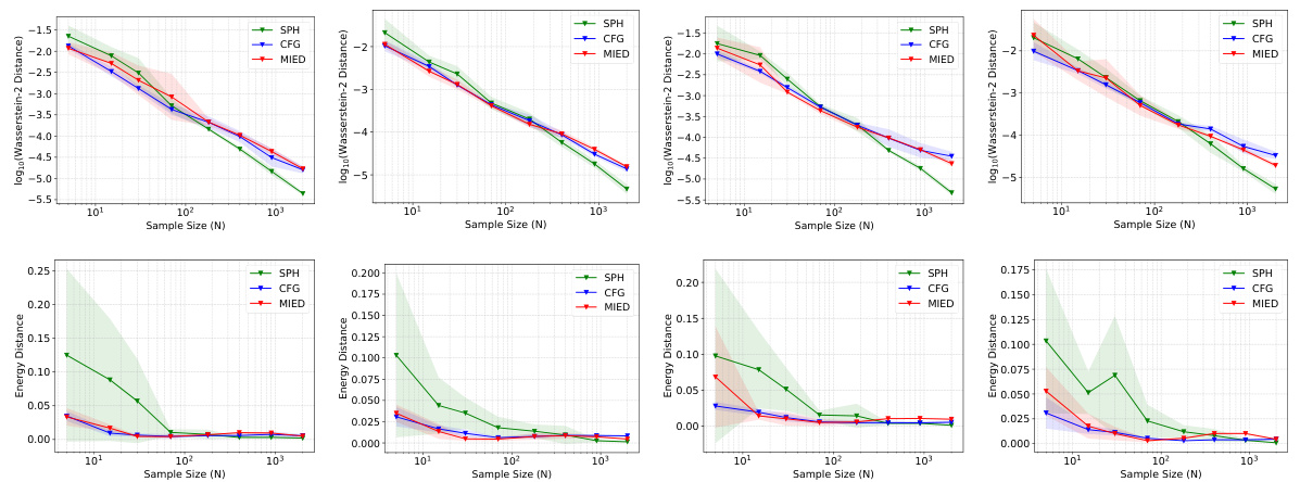
🔼 This figure presents the mean squared error (MSE) of the band-wise approximation of the boundary integral for three different velocity fields (v1, v2, v3) and three different distributions (p1, p2, p3). The x-axis represents the sample size (N), and the y-axis represents the log10(MSE). Each plot shows how the MSE decreases as the sample size increases for each combination of velocity and distribution. This illustrates the accuracy and convergence of the boundary integral estimation method used in the paper.
read the caption
Figure 4: Left: MSE of boundary integral estimation of distribution p1. Middle: MSE of boundary integral estimation of distribution p2. Right: MSE of boundary integral estimation of distribution p3.
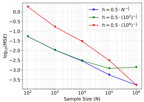
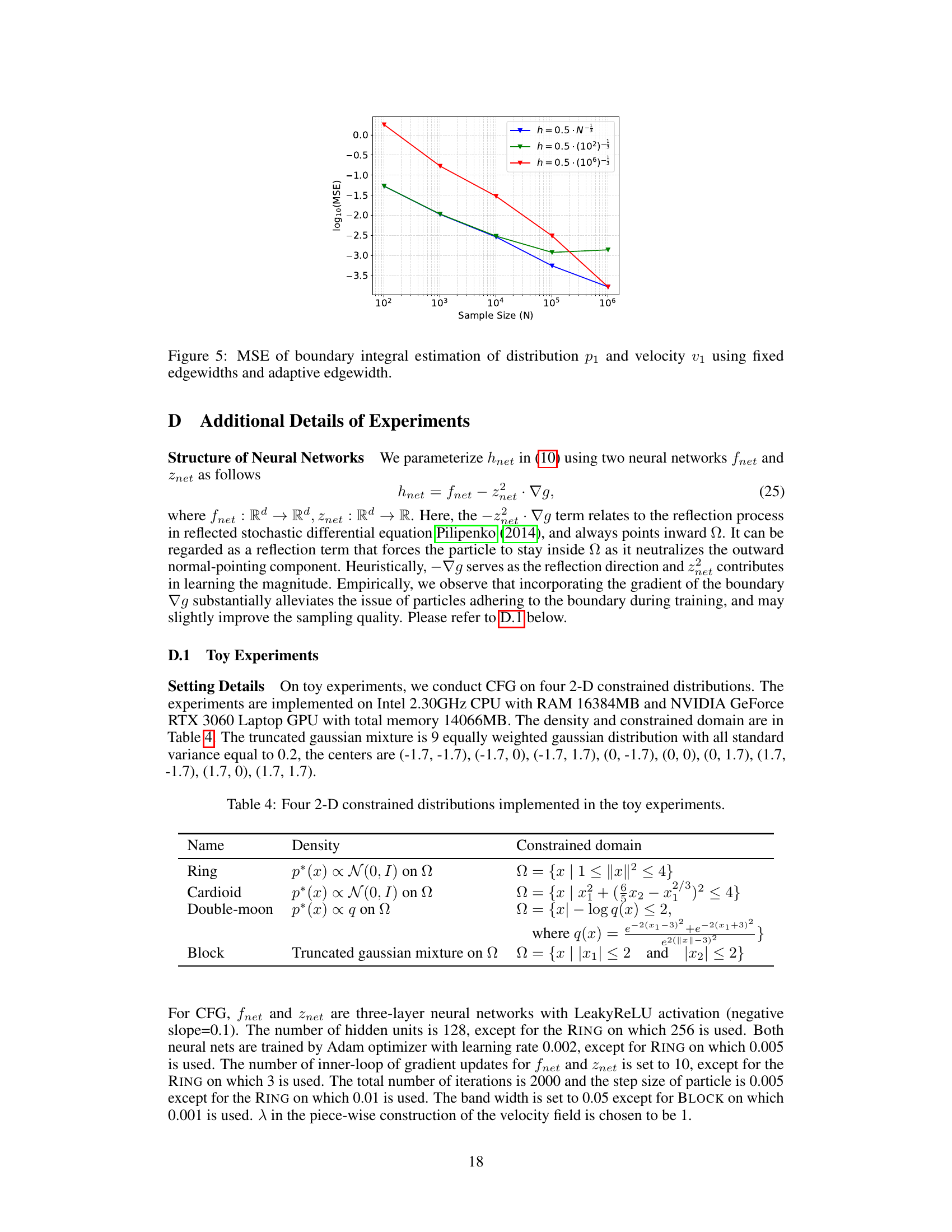
🔼 This figure demonstrates the Mean Squared Error (MSE) of the boundary integral estimation method used in the paper. Three different bandwidths are compared: a fixed bandwidth of 0.5, a fixed bandwidth of 0.5*(10^2)^(-1/3), and an adaptive bandwidth of 0.5*N^(-1/3), where N is the sample size. The plot shows how the MSE changes as the sample size increases. The adaptive bandwidth shows better performance in terms of lower MSE across varying sample sizes.
read the caption
Figure 5: MSE of boundary integral estimation of distribution p₁ and velocity v₁ using fixed edgewidths and adaptive edgewidth.

🔼 This figure compares the sampling results of three ablation studies on four different constrained 2D distributions (ring, cardioid, double-moon, block) against the ground truth. The ablation studies involve: (1) not estimating the boundary integral, (2) not using znet, and (3) using znet. The visualization helps understand how each of these components affects the performance of the constrained sampling method. The results show that using znet and estimating the boundary integral are both crucial for accurate results.
read the caption
Figure 6: Ablation sampling results of not estimating boundary integral (left), not using znet (middle left), using znet (middle right) and the ground truth (right).

🔼 The figure shows the results of applying the proposed method to a 3D ring-shaped distribution. The initial distribution is a 3D standard Gaussian. The particles are constrained to lie on the xOy plane (equality constraint: z = 0) and within a ring in the xOy plane (inequality constraint: 1 < x² + y² < 4). The figure displays the particle positions at iterations 0, 100, and 1000, showing how the particles converge to the target distribution while satisfying both constraints. The ground truth distribution is also shown.
read the caption
Figure 7: Illustration of generalizing our method to accommodating equality and inequality constraints.
🔼 This figure shows the performance of the proposed Constrained Functional Gradient Flow (CFG) method for sampling from truncated Gaussian distributions within various constrained domains. The left panel displays the particle distribution at different iteration numbers for ring-shaped, cardioid-shaped, double-moon-shaped, and block-shaped domains, illustrating how the particles converge to the target distribution without escaping the domain. The right panel compares the convergence curves of CFG with MSVGD and MIED on a block-shaped domain using Wasserstein-2 distance and energy distance metrics. This demonstrates that CFG effectively handles constraints and achieves better sampling results compared to other baselines.
read the caption
Figure 1: Left: CFG sampled particles at different numbers of iterations on constrained domains (ring, cardioid, double-moon, block). Right: The convergence curves of MSVGD, CFG and MIED on the block constraint.

🔼 This figure compares the performance of CFG and MIED in terms of Wasserstein-2 distance against training time for different numbers of particles (900, 2000, and 4000). It demonstrates the scalability of CFG compared to MIED, showing that CFG’s training time increases linearly with the number of particles while MIED’s increases quadratically. This is because the complexity of CFG is O(N) while MIED’s is O(N^2), where N is the number of particles. The figure highlights the superior computational efficiency of CFG, especially for larger datasets.
read the caption
Figure 9: Wasserstein-2 distance of CFG and MIED versus the training time using different number of particles.
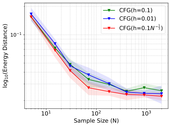
🔼 This figure compares the performance of the proposed CFG method using different bandwidth selection strategies for the Bayesian Lasso problem. It shows the energy distance (a measure of the difference between the estimated and true distributions) plotted against the sample size (number of particles) for three different bandwidth methods: a fixed bandwidth of 0.1, a fixed bandwidth of 0.01, and an adaptive bandwidth of 0.1N⁻³. The adaptive bandwidth, represented in red, generally shows better performance (lower energy distance) across different sample sizes. This supports the claim that the adaptive bandwidth selection method is more effective for the Bayesian Lasso problem.
read the caption
Figure 10: Choosing the adaptive bandwidth (red) against fixed bandwidths for the Bayesian Lasso experiment on a synthetic dataset.
More on tables

🔼 This table lists the types of velocities and probability distributions used in the verification experiment of the boundary integral estimation. Three types of velocities and three types of distributions are considered. The velocities are vector fields, and the distributions are either uniform or Gaussian distributions, each defined within the constrained domain Ω.
read the caption
Table 2: The types of velocities and distributions.

🔼 This table shows the true values of the boundary integral used in the simulation study to verify the accuracy of the band-wise approximation method for estimating the boundary integral in the constrained domain sampling problem. Three different velocity fields (v1, v2, v3) and three different probability distributions (p1, p2, p3) are considered. The values in the table represent the true values of the boundary integral for each combination of velocity field and distribution. This data is used to compare against the approximated values calculated using the proposed method, assessing its accuracy in approximating the boundary integral.
read the caption
Table 3: The true values of boundary integral in the verification experiment.

🔼 This table lists four 2D constrained distributions used in the toy experiments of the paper. For each distribution, it provides the name, probability density function (defined up to a proportionality constant), and the mathematical description of the constrained domain (Ω). The distributions represent different shapes of constrained regions, including a ring, cardioid, double-moon, and a block.
read the caption
Table 4: Four 2-D constrained distributions implemented in the toy experiments.

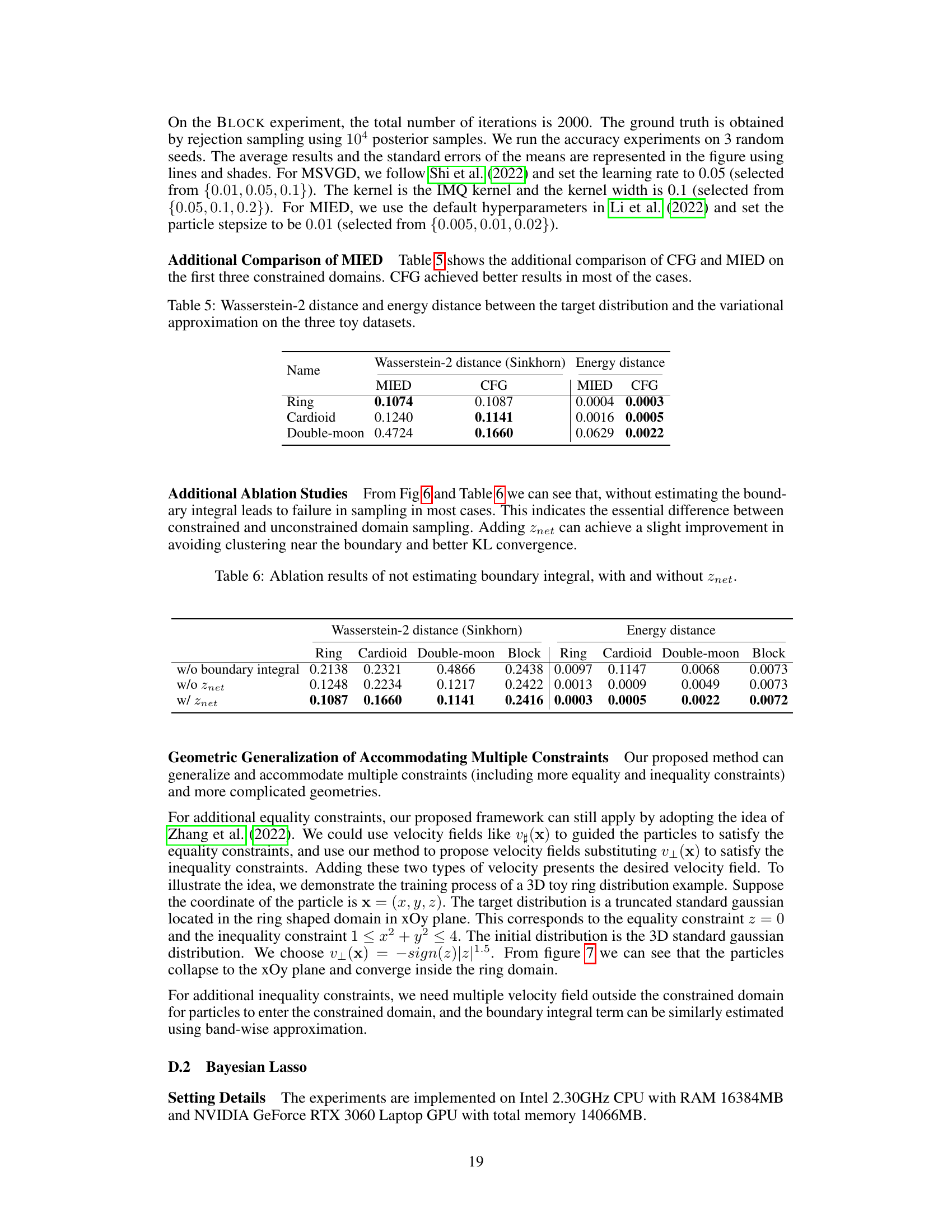
🔼 This table presents a comparison of the Wasserstein-2 distance and energy distance between the target distribution and the approximation achieved by MIED and CFG methods on three different 2D constrained distributions (Ring, Cardioid, and Double-moon). The results show that CFG generally outperforms MIED in terms of both metrics, indicating its superior approximation capability for these specific tasks.
read the caption
Table 5: Wasserstein-2 distance and energy distance between the target distribution and the variational approximation on the three toy datasets.

🔼 This table presents ablation study results comparing the performance of the proposed CFG method with and without two key components: boundary integral estimation and the Znet neural network. It shows the Wasserstein-2 distance and energy distance for four different toy datasets (Ring, Cardioid, Double-moon, Block) under three different settings: without boundary integral estimation, without Znet, and with both Znet and boundary integral estimation. The results demonstrate the importance of both components for effective constrained sampling.
read the caption
Table 6: Ablation results of not estimating boundary integral, with and without Znet.

🔼 This table presents the results of a larger monotonic Bayesian neural network experiment on the COMPAS dataset. It compares different methods (PD-SVGD, C-SVGD, MIED, and CFG) under varying monotonicity thresholds (0.05, 0.01, 0.005). The metrics evaluated are test accuracy, test negative log-likelihood (NLL), and the ratio of particles outside the constrained domain. The best and second-best results for each threshold are highlighted, along with any instances where a significant proportion of particles fall outside the constrained region.
read the caption
Table 7: Results of a larger monotonic Bayesian neural network on COMPAS dataset under different monotonicity threshold. The results are averaged from the last 10 checkpoints for robustness. For each monotonicity threshold, the best result is marked in black bold font and the second best result is marked in brown bold font. Positive proportion of particles outside the constrained domain is marked in red.

🔼 This table presents the results of a monotonic Bayesian neural network on a high-dimensional dataset (Blog Feedback, 276 dimensions). The model uses 13903 particles. The results (test RMSE and ratio of particles outside the constrained domain) are averaged over the last 10 checkpoints to ensure robustness and reliability. It shows the performance of different methods on this challenging high-dimensional problem.
read the caption
Table 8: Results of monotonic BNN on a higher 276-dimensional dataset Blog Feedback. The particle dimension is 13903. The results are averaged from the last 10 checkpoints for robustness.
Full paper#

