TL;DR#
Key Takeaways#
Why does it matter?#
This paper is crucial for researchers in generative modeling and optimal transport. It offers a novel approach to learn flows with straight trajectories, solving a key challenge in FM methods. This efficiency improvement opens new avenues for developing faster and more accurate generative models, advancing the field significantly. The theoretical justifications and readily available codebase further enhance its impact.
Visual Insights#
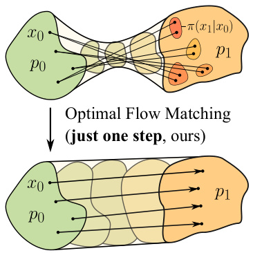
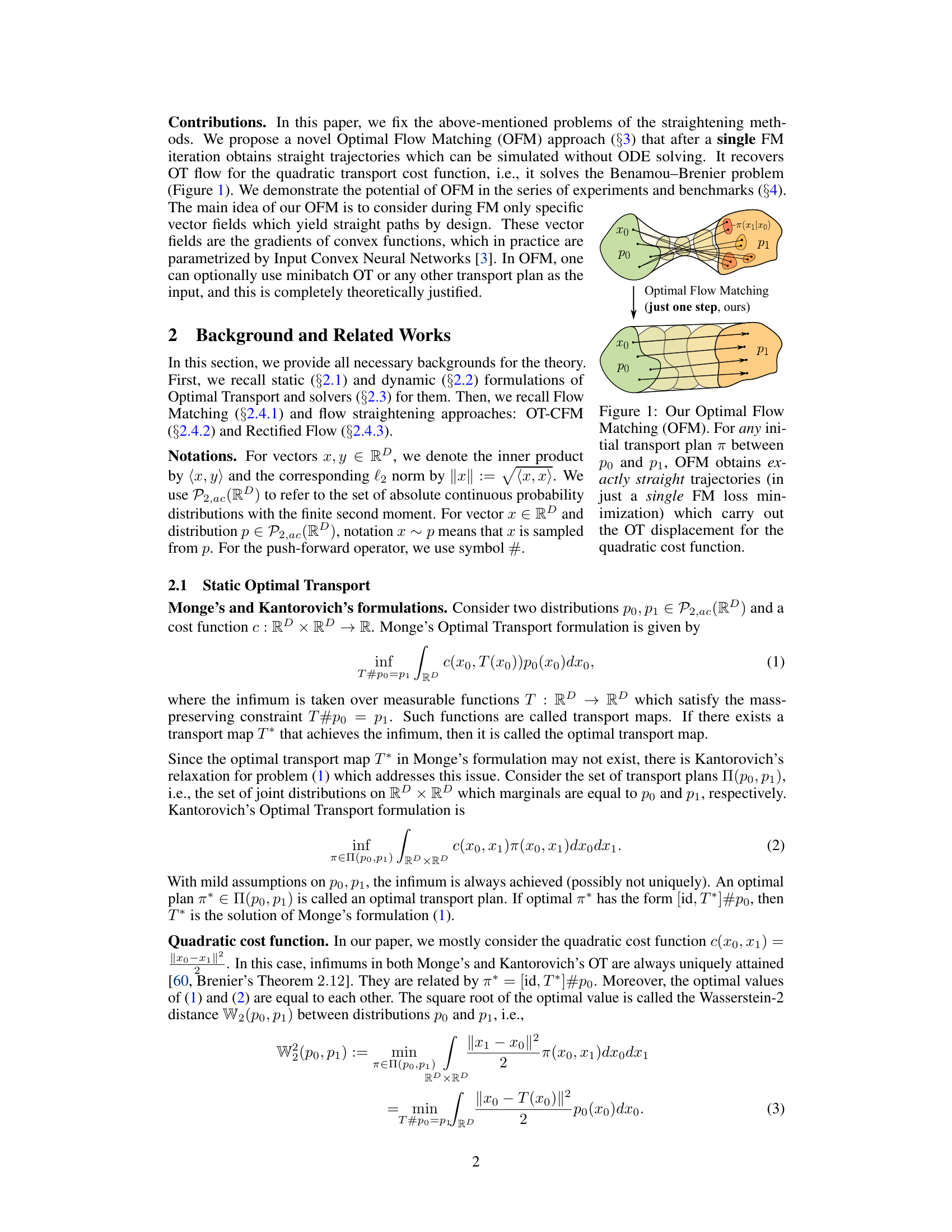
🔼 This figure illustrates the core idea of the Optimal Flow Matching (OFM) method. It shows how, starting with an arbitrary initial transport plan (a way to map points from the source distribution p₀ to the target distribution p₁), OFM achieves straight trajectories in a single step that precisely solve the optimal transport problem for quadratic cost. In contrast to other methods that use iterative procedures and might produce curved trajectories, OFM leverages convex functions to directly produce straight paths.
read the caption
Figure 1: Our Optimal Flow Matching (OFM). For any initial transport plan π between po and p1, OFM obtains exactly straight trajectories (in just a single FM loss minimization) which carry out the OT displacement for the quadratic cost function.
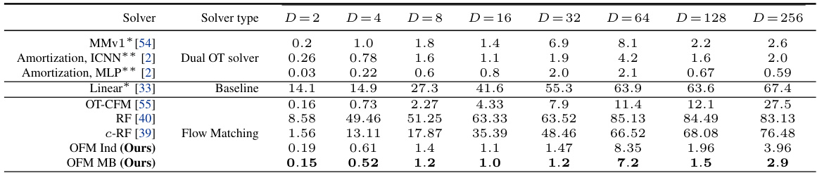
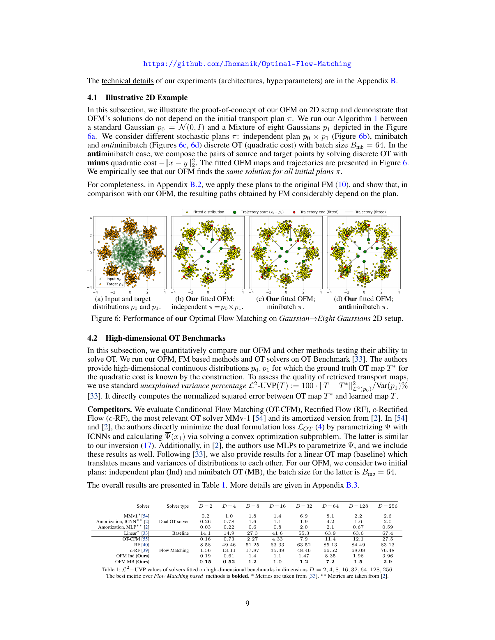
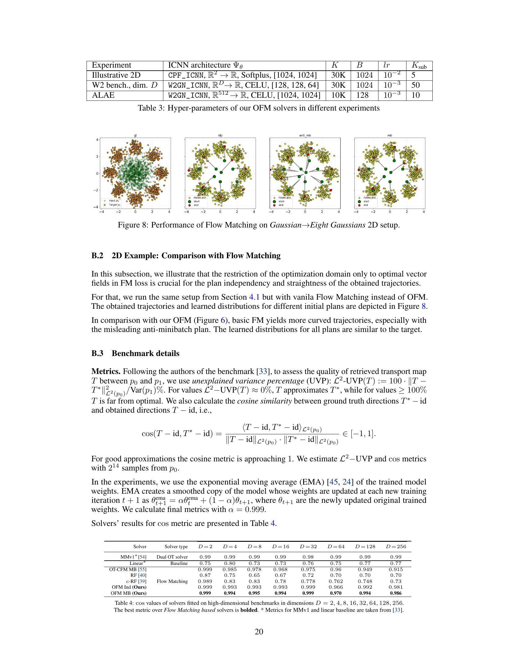
🔼 This table presents the results of various optimal transport solvers on a high-dimensional benchmark. The L2-UVP (unexplained variance percentage) metric measures the error between the learned transport map and the ground truth map. Lower values indicate better performance. The table compares different Flow Matching methods (OT-CFM, RF, c-RF, OFM) against other OT solvers (MMv1, Amortization with ICNN, Amortization with MLP) and a linear baseline. The results are shown for different dimensions (D).
read the caption
Table 1: L2−UVP values of solvers fitted on high-dimensional benchmarks in dimensions D = 2, 4, 8, 16, 32, 64, 128, 256. The best metric over Flow Matching based methods is bolded. * Metrics are taken from [33]. ** Metrics are taken from [2].
In-depth insights#
Optimal Flow Match#
Optimal flow matching presents a novel approach to generative modeling, addressing limitations of existing methods. It leverages the concept of straight trajectories in optimal transport, offering faster inference and avoiding error accumulation during training. By parameterizing vector fields with convex functions, specifically gradients of convex functions, the method ensures that the learned flow directly recovers the optimal transport map for quadratic cost functions. This is achieved in a single step, eliminating the iterative refinement needed in previous methods like rectified flow. The theoretical justification provides a solid foundation for the approach, demonstrating equivalence between the proposed loss function and the optimal transport dual formulation. Computational experiments highlight OFM’s effectiveness, showing superior performance compared to existing techniques in terms of both accuracy and efficiency. While OFM currently focuses on quadratic cost functions, its underlying principles suggest potential extensions to more general cost functions.
Straight Trajectories#
The concept of “straight trajectories” in the context of optimal transport and flow matching is crucial for efficiency. Straight trajectories drastically reduce the computational cost associated with integrating ordinary differential equations (ODEs), a common step in generative modeling. The paper explores methods to achieve this. While iterative approaches exist, they suffer from error accumulation. A novel approach, Optimal Flow Matching (OFM), is proposed, aiming to directly learn straight trajectories in a single step by employing specific vector fields parameterized by convex functions. This one-step method offers a significant advantage in speed and computational efficiency over iterative techniques and successfully addresses the limitations of prior methods. The theoretical justification and experimental validation of OFM demonstrate its effectiveness in generating flows with straight trajectories, making it a significant contribution to the field of generative modeling and optimal transport.
Single-Step OFM#
The concept of “Single-Step OFM” suggests a significant advancement in optimal transport (OT) and flow matching (FM) by achieving accurate OT solutions in just one step, unlike iterative methods. This is particularly valuable as it eliminates error accumulation inherent in iterative approaches like Rectified Flow. The key innovation likely lies in carefully selecting and parameterizing the vector fields used in the FM process, possibly using the gradients of convex functions. This constraint cleverly guides the flow towards straight trajectories, directly mapping the initial distribution to the target distribution. Computational efficiency is a major benefit, as solving the OT problem in a single step drastically reduces runtime. While the method might be currently limited to specific cost functions, its theoretical foundation and empirical success suggest a potentially transformative impact on generative modeling, improving the efficiency and accuracy of generative processes that rely on optimal transport.
High-dim Benchmarks#
The high-dimensional benchmark section likely evaluates the performance of the proposed Optimal Flow Matching (OFM) method against existing Optimal Transport (OT) solvers and other flow matching techniques on datasets with high-dimensional features. The results would demonstrate OFM’s scalability and accuracy in solving OT problems in complex, high-dimensional spaces. Key aspects to consider include the choice of metrics used to assess the quality of the learned transport maps, the types of high-dimensional distributions used in the benchmark, and the computational cost of OFM compared to competing methods. It is also expected that the benchmark would showcase OFM’s advantage in achieving straight trajectories, leading to potential improvements in efficiency and accuracy, especially when dealing with high-dimensional data where curved trajectories are common.
Future Directions#
Future research could explore extending Optimal Flow Matching (OFM) to handle more general cost functions beyond the quadratic case, potentially leveraging insights from entropic optimal transport. Improving the efficiency of the flow map inversion is crucial, as it currently forms a computational bottleneck. Investigating alternative optimization strategies beyond LBFGS, such as those tailored for strongly convex problems, could significantly reduce computational costs. Exploring alternative parametrizations for the convex functions in OFM, moving beyond Input Convex Neural Networks (ICNNs) to potentially more expressive architectures, is another avenue for improvement. Finally, a deeper theoretical analysis could investigate the convergence properties of OFM and its relationship to other optimal transport methods, providing a more robust theoretical foundation. Combining OFM with other generative modeling techniques, such as diffusion models, could lead to exciting new generative models.
More visual insights#
More on figures
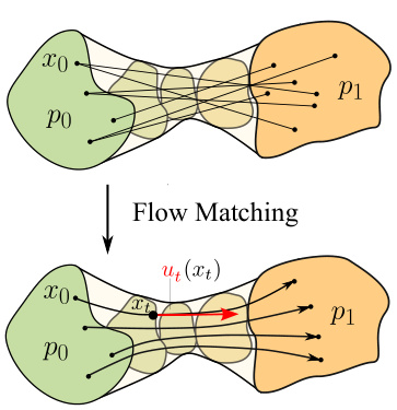
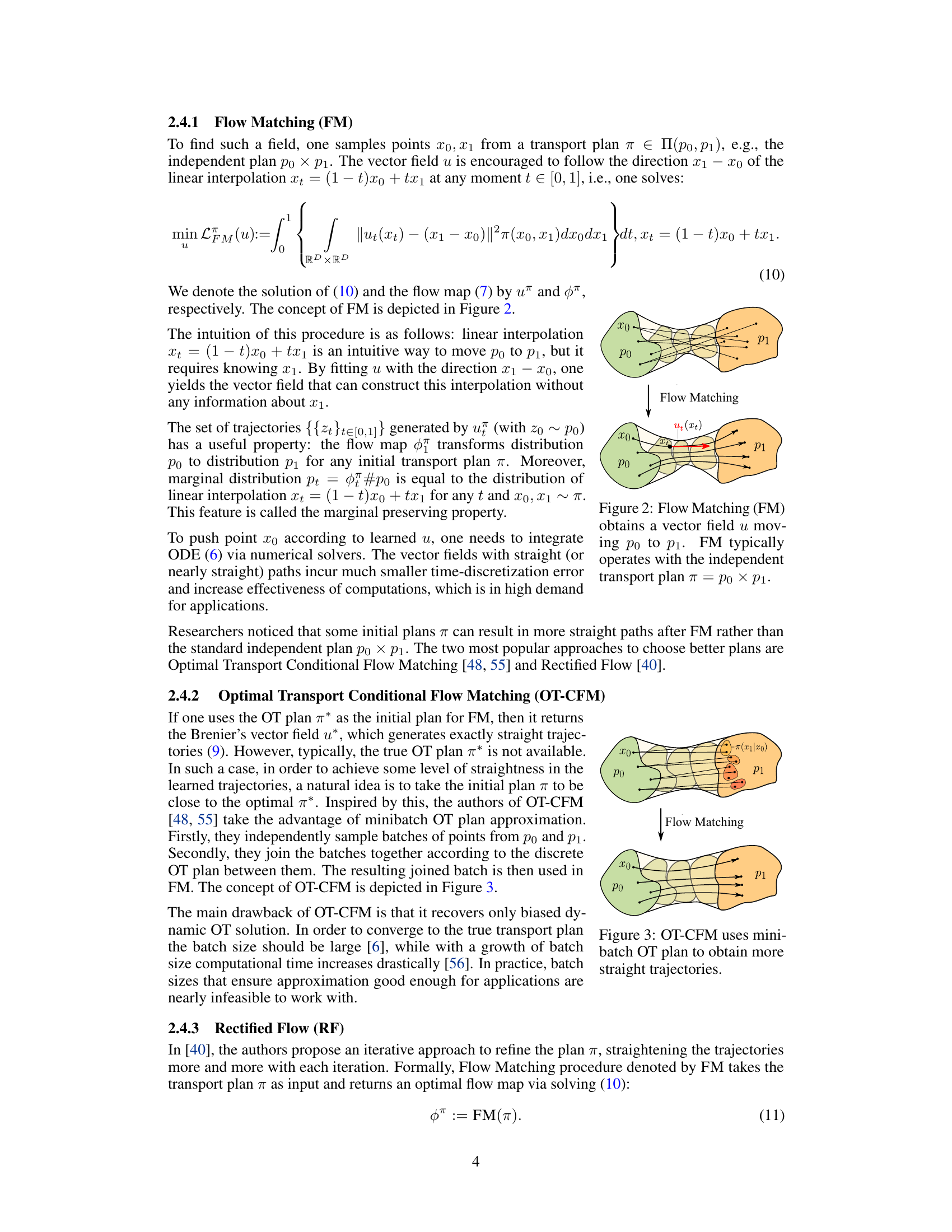
🔼 This figure illustrates the concept of Flow Matching (FM). It shows two probability distributions, p0 (green) and p1 (orange), and samples drawn from them. Initially, there are direct connections between samples from p0 and p1. The FM algorithm then finds a vector field, represented by the red arrow, that aims to move points from distribution p0 to p1. This vector field aims to align the movement with the direction connecting each pair of samples from the original distributions, making the trajectories more direct, ideally straight lines. The resulting transport plan is often not the true optimal transport plan.
read the caption
Figure 2: Flow Matching (FM) obtains a vector field u moving po to p1. FM typically operates with the independent transport plan π = po × p1.
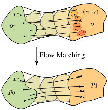
🔼 This figure illustrates the concept of Flow Matching (FM). It shows two probability distributions, po (green) and p1 (orange), connected by a transport plan π, represented by lines connecting points from po to p1. FM aims to find a vector field u that moves po to p1. The independent transport plan π = po × p1 is a simple case where each point in po is independently connected to a point in p1, as shown by the lines. The resulting flow is depicted below, where the vector field u guides the points of po towards p1.
read the caption
Figure 2: Flow Matching (FM) obtains a vector field u moving po to p1. FM typically operates with the independent transport plan π = po × p1.
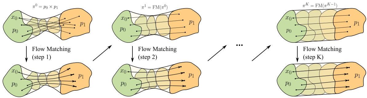
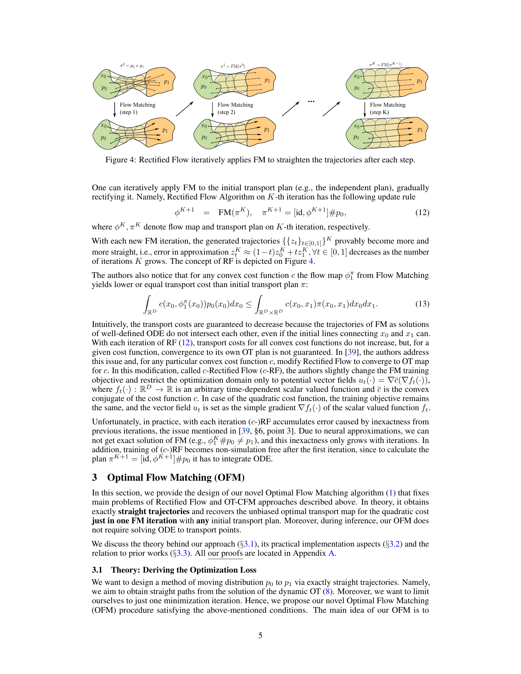
🔼 Rectified Flow is an iterative method that refines the transport plan by applying Flow Matching repeatedly. The initial transport plan (e.g., independent plan) is gradually rectified. In each iteration, Flow Matching (FM) is applied to the current transport plan (πk) to generate a new flow map (φk+1). This flow map is then used to update the transport plan (πk+1) for the next iteration. This process continues for K iterations. With each iteration, the trajectories generated by the flow map become increasingly straight, improving the approximation of the Optimal Transport (OT) map. The figure depicts this process visually, showing the trajectories becoming more aligned between the initial distribution and the target distribution as the number of iterations (k) increases.
read the caption
Figure 4: Rectified Flow iteratively applies FM to straighten the trajectories after each step.
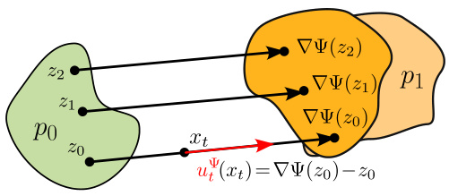
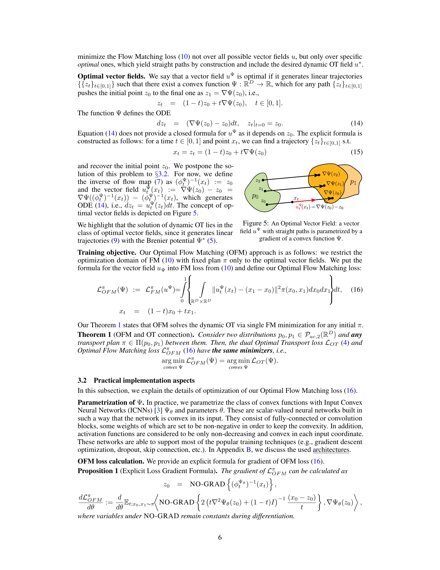
🔼 This figure illustrates the concept of an optimal vector field in the context of Optimal Flow Matching. It shows how a vector field, denoted as u, can be parameterized by the gradient of a convex function, Ψ. The key feature is that this specific type of vector field, by its design, will always generate straight trajectories (paths) when used to transport probability distributions. The figure displays sample points (z0, z1, z2) from an initial distribution (p0) being transported to corresponding points in the target distribution (p1) along straight lines. The vector field u(xt) is calculated at any point xt, based on the inverse of the flow map φ-1(xt), which recovers the origin point z0 along the straight path. This property is crucial for the efficiency and accuracy of the Optimal Flow Matching algorithm.
read the caption
Figure 5: An Optimal Vector Field: a vector field u with straight paths is parametrized by a gradient of a convex function Ψ.
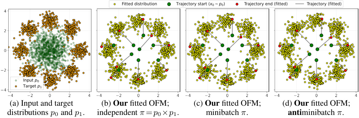
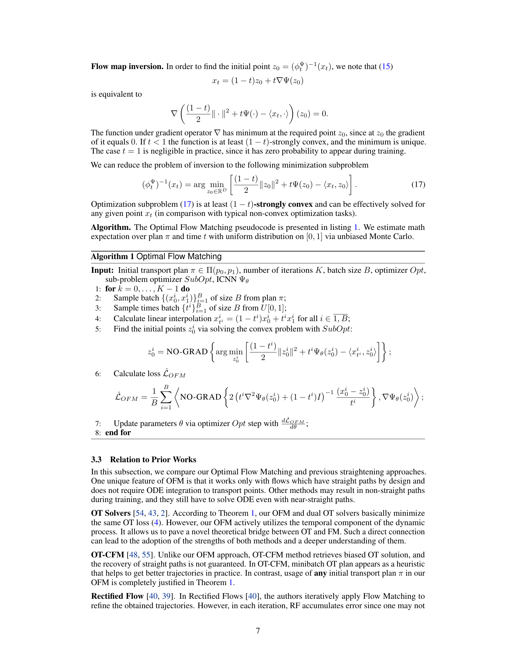
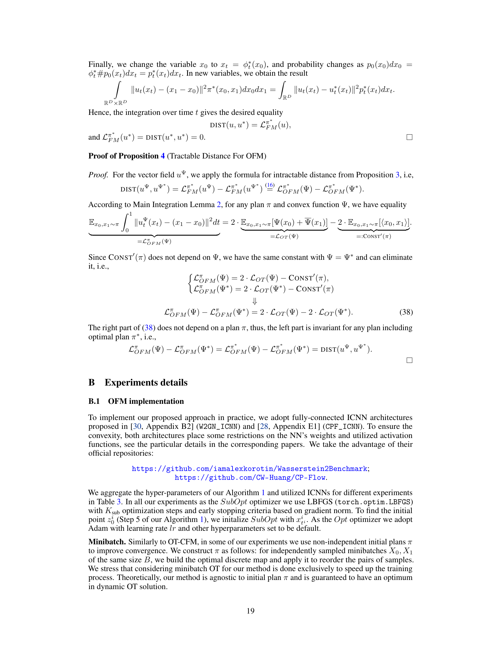
🔼 This figure shows the results of applying the Optimal Flow Matching (OFM) algorithm to a simple 2D problem involving a Gaussian source distribution and a target distribution consisting of eight Gaussians. It demonstrates the algorithm’s performance with different initial transport plans π. (b) illustrates OFM’s performance when using an independent initial plan (π = p₀ × p₁). (c) and (d) show the results obtained with minibatch and antiminibatch plans, respectively. The plots show the input and target distributions, the learned trajectories, and the final distribution obtained by the OFM. The consistent results across different initial plans highlight the robustness of the OFM.
read the caption
Figure 6: Performance of our Optimal Flow Matching on Gaussian Eight Gaussians 2D setup.
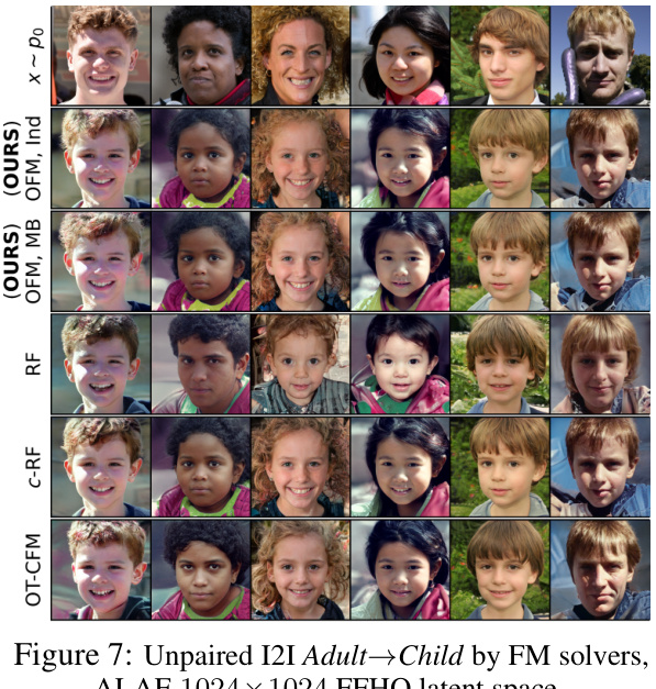
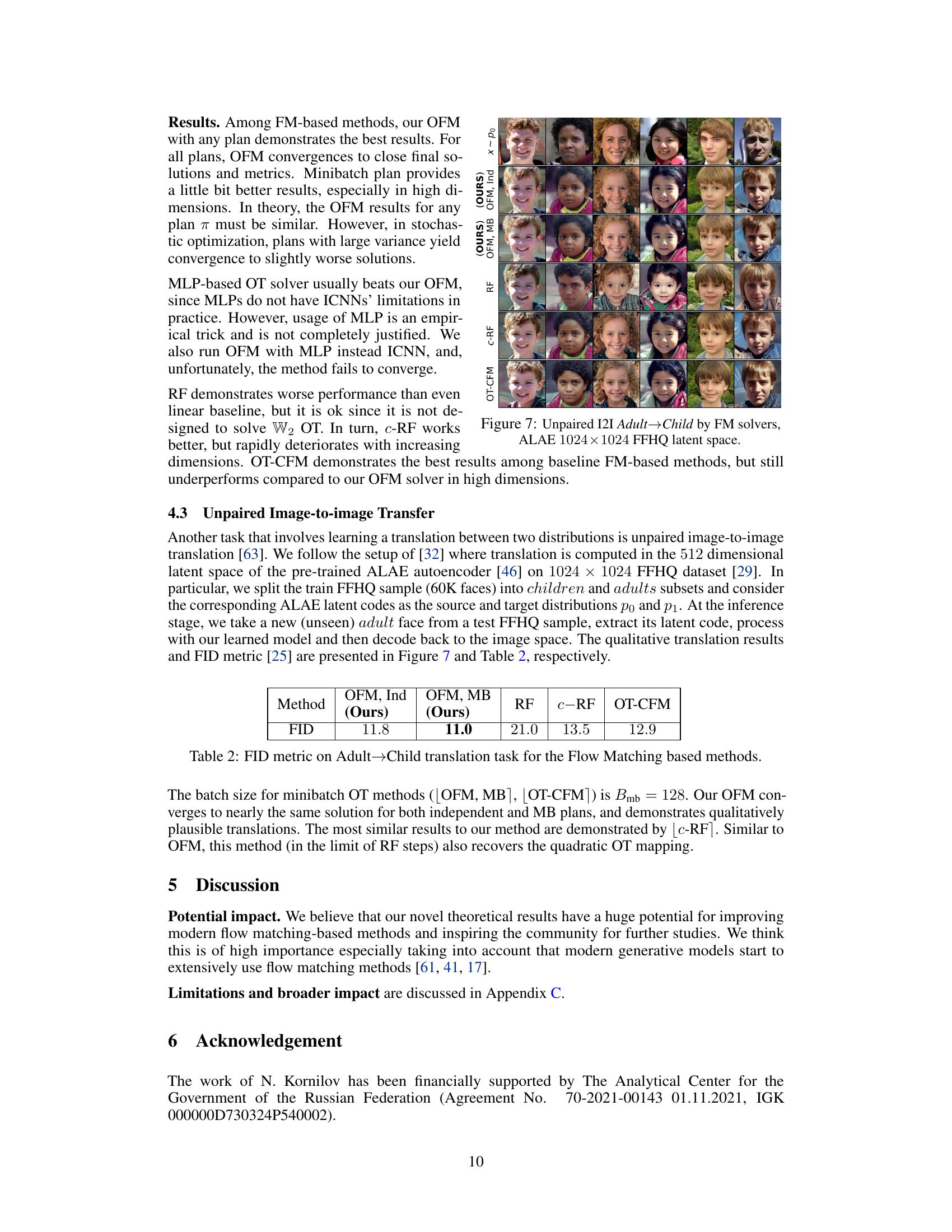
🔼 This figure shows the results of unpaired image-to-image translation using different flow matching methods. The goal is to translate adult faces into child faces in the latent space of a pretrained ALAE autoencoder. The figure displays sample images generated by the OFM (ours), RF, c-RF, and OT-CFM methods, demonstrating the visual quality and differences in generated child faces produced by each method.
read the caption
Figure 7: Unpaired I2I Adult→Child by FM solvers, ALAE 1024 × 1024 FFHQ latent space.
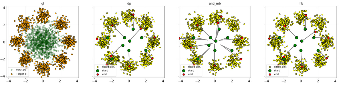
🔼 This figure shows the results of applying Optimal Flow Matching (OFM) to a 2D problem with different initial transport plans. The input distribution is a standard Gaussian, and the target distribution is a mixture of eight Gaussians. The figure shows that OFM obtains similar results for various plans, indicating plan independence, a key advantage of the proposed method.
read the caption
Figure 6: Performance of our Optimal Flow Matching on Gaussian Eight Gaussians 2D setup.
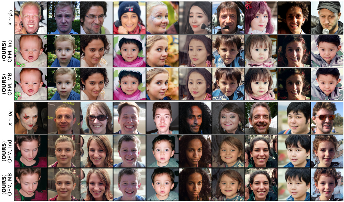
🔼 This figure shows the results of unpaired image-to-image translation using different flow matching methods (OT-CFM, RF, c-RF, and OFM) in the latent space of a pretrained ALAE autoencoder. The top row displays the input adult images. Subsequent rows show the results of translating those adult images into child images using the indicated method. The results demonstrate the ability of the OFM approach to produce more realistic and coherent child images compared to the other methods.
read the caption
Figure 7: Unpaired I2I Adult→Child by FM solvers, ALAE 1024 × 1024 FFHQ latent space.
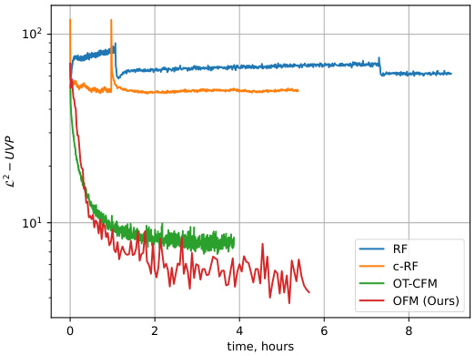
🔼 The figure shows the L²-UVP metric (a measure of the quality of the retrieved transport maps) plotted against training time (in hours) for various methods: RF, c-RF, OT-CFM, and OFM. It illustrates how quickly each method approaches the optimal transport map, with OFM demonstrating faster convergence. The y-axis is on a logarithmic scale, highlighting the difference in convergence speed between methods.
read the caption
Figure 10: L²-UVP metric depending on the elapsed training time in dimension D = 32.
More on tables
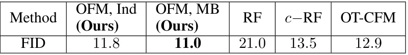
🔼 This table presents the Fréchet Inception Distance (FID) scores for different flow matching based methods on the Adult Child image-to-image translation task. The FID score is a common metric for evaluating the quality of generated images, with lower scores indicating better image quality. The results show that the proposed Optimal Flow Matching (OFM) method achieves the lowest FID score, indicating superior performance compared to other methods such as Rectified Flow (RF), c-Rectified Flow (c-RF), and Optimal Transport Conditional Flow Matching (OT-CFM).
read the caption
Table 2: FID metric on Adult Child translation task for the Flow Matching based methods.

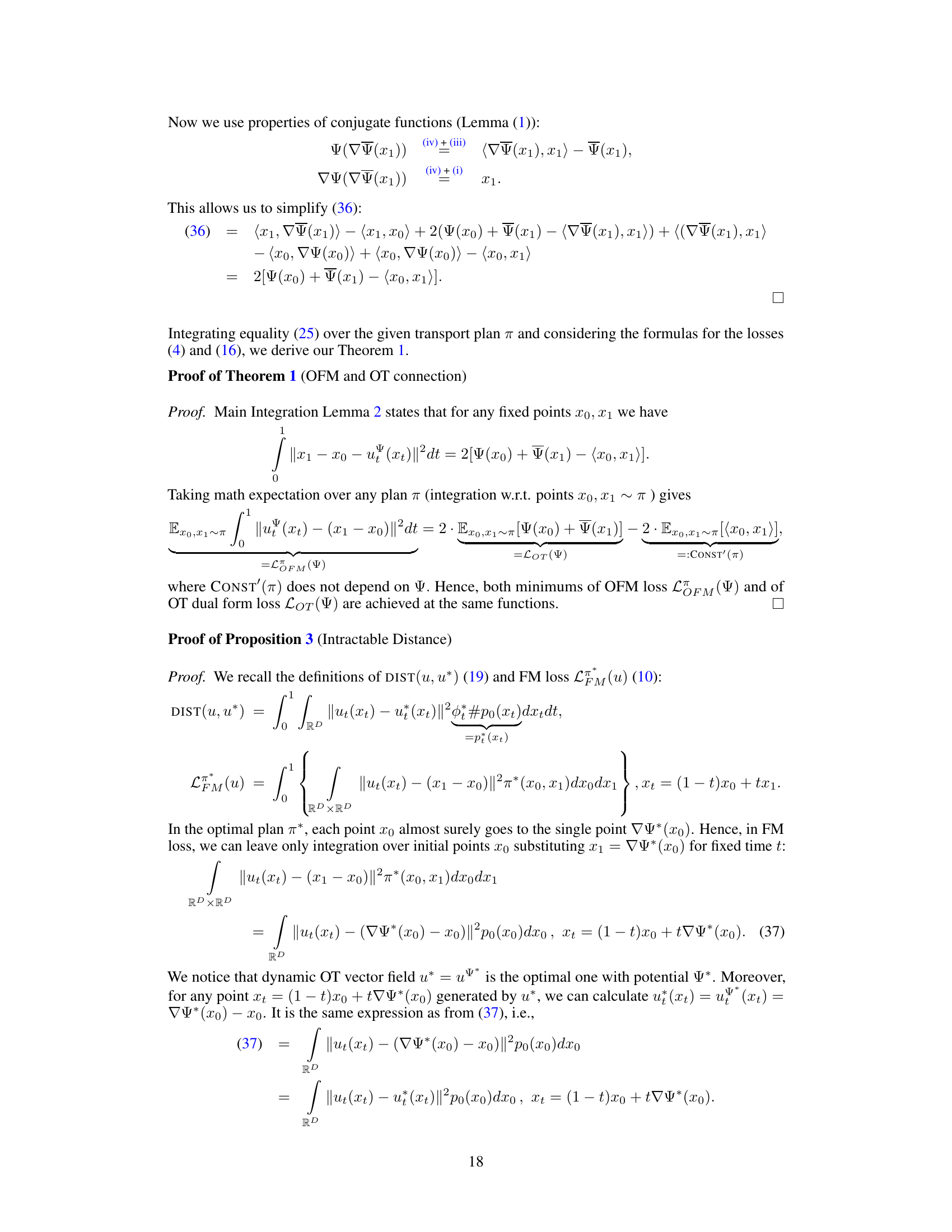
🔼 This table presents the hyperparameters used in the Optimal Flow Matching (OFM) experiments for three different scenarios: Illustrative 2D, Wasserstein-2 benchmark with varying dimensions (D), and unpaired image-to-image transfer using ALAE. For each scenario, the table specifies the ICNN architecture used for parametrizing the convex function Ψ, the number of iterations (K), batch size (B), learning rate (lr), and the number of sub-problem optimization steps (Ksub).
read the caption
Table 3: Hyper-parameters of our OFM solvers in different experiments
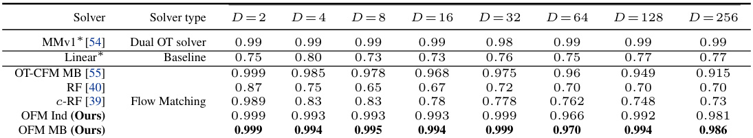
🔼 This table presents the results of applying various Optimal Transport (OT) solvers to high-dimensional benchmark datasets. The performance is measured using the L2-UVP metric, which quantifies the error between the learned OT map and the ground truth OT map. Solvers include both traditional OT methods and Flow Matching (FM)-based approaches. The table allows a comparison of the accuracy and efficiency of these different OT solving methods across different dimensions.
read the caption
Table 1: L2-UVP values of solvers fitted on high-dimensional benchmarks in dimensions D = 2, 4, 8, 16, 32, 64, 128, 256. The best metric over Flow Matching based methods is bolded. * Metrics are taken from [33]. ** Metrics are taken from [2].
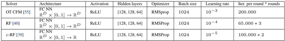
🔼 This table presents the architectures and hyperparameters of the neural networks used for the competing Flow Matching methods (OT-CFM, RF, c-RF) in the high-dimensional OT benchmark experiments. It details the network architecture (fully connected), activation function (ReLU), number of hidden layers, optimizer used (RMSProp), batch size, learning rate, and the number of iterations per round multiplied by the total number of rounds.
read the caption
Table 5: Parameters of models fitted on benchmark in dimensions D = 2, 4, 8, 16, 32, 64, 128, 256.
Full paper#