↗ arXiv ↗ Hugging Face ↗ Hugging Face ↗ Chat
TL;DR#
Creating effective text embeddings from large language models (LLMs) is computationally expensive. Existing methods lack systematic guidance on optimizing model parameters and training strategies to balance performance and resource usage. This often leads to suboptimal models and wasted resources.
This paper introduces an algorithm that determines the best combination of model size, training data, and fine-tuning techniques for any given computational budget. Through extensive experimentation, it identifies specific fine-tuning methods that are optimal at different budget levels and provides scaling laws to predict optimal performance for various model configurations. This makes the design process easier for practitioners and ensures they get the best possible embedding models without exceeding resource limits.
Key Takeaways#
Why does it matter?#
This paper is crucial for researchers working with large language models and text embeddings. It provides a practical algorithm and readily applicable scaling laws, enabling efficient fine-tuning for optimal performance even with limited computational resources. This directly addresses a major challenge in the field, reducing costs and improving model efficiency. The open-sourced code further enhances reproducibility and facilitates broader adoption of the findings.
Visual Insights#
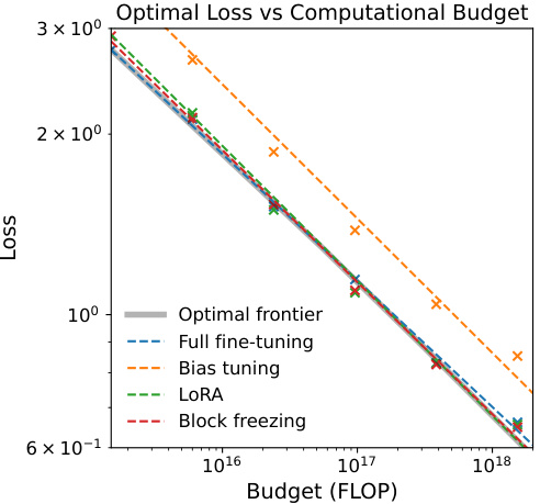
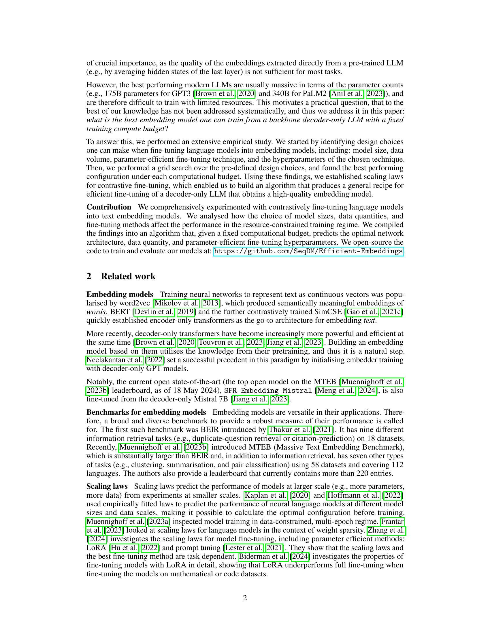
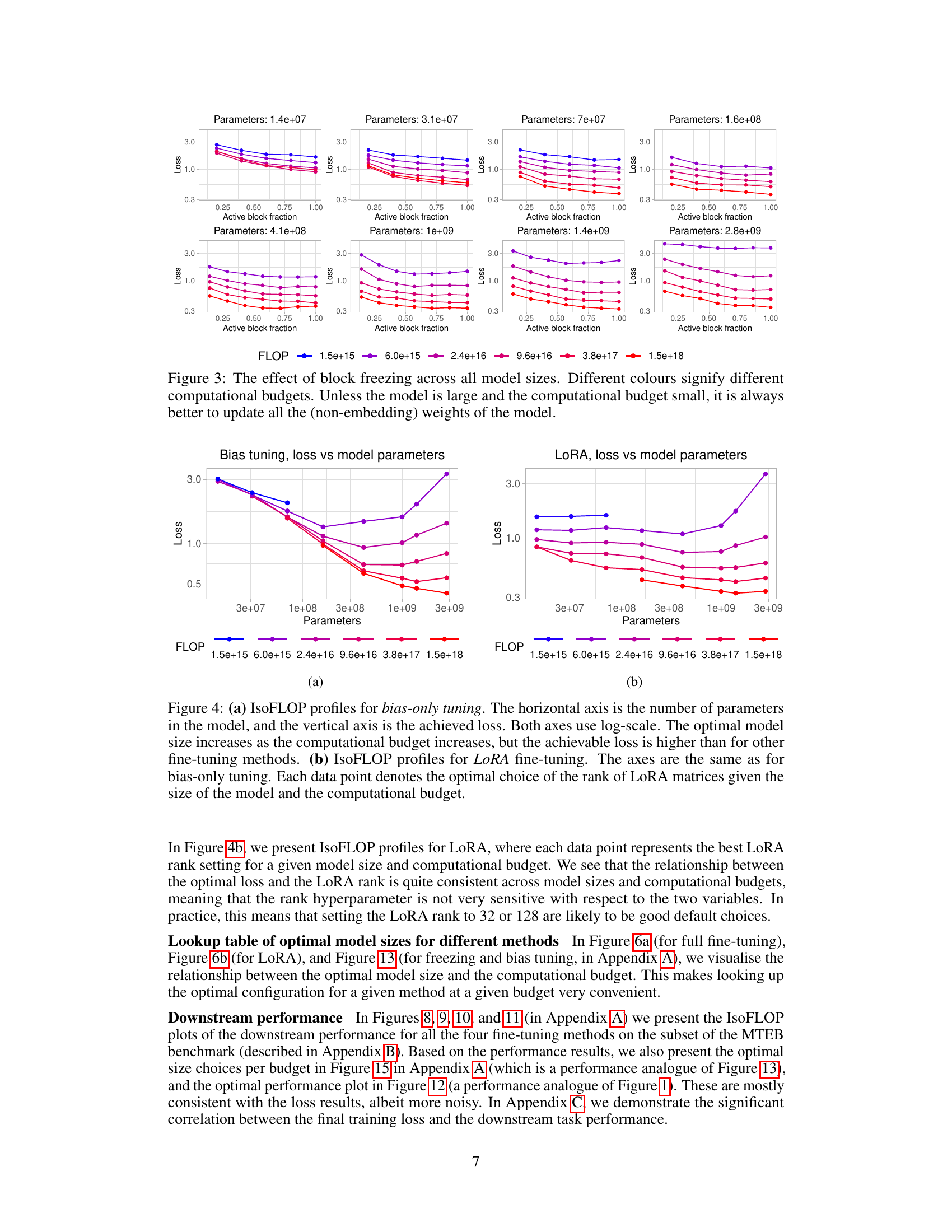
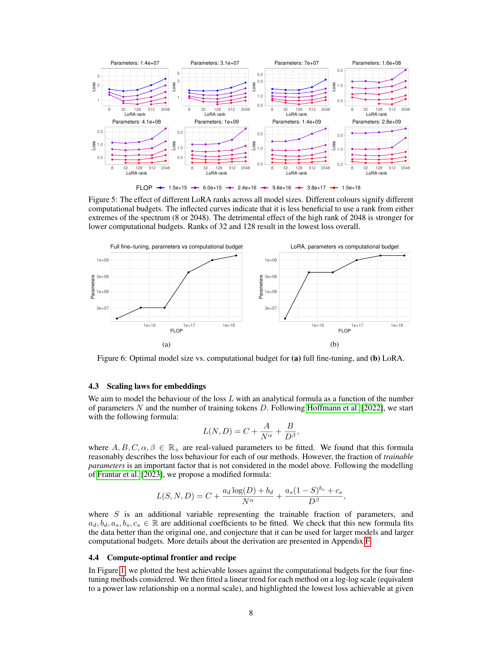
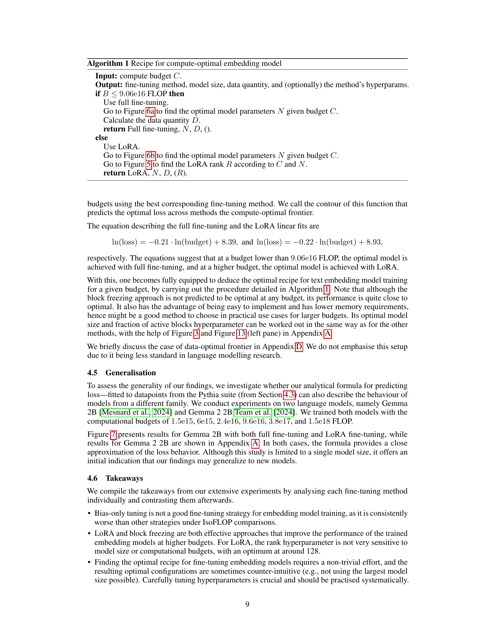
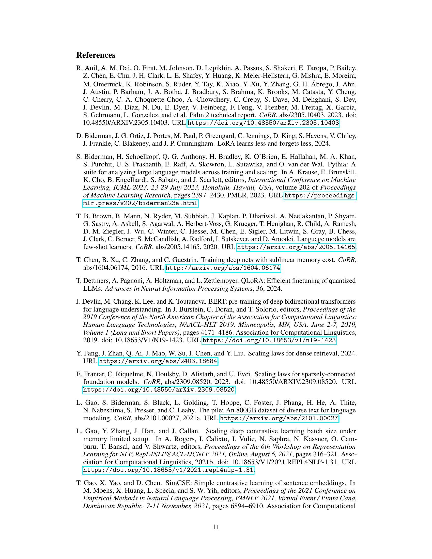
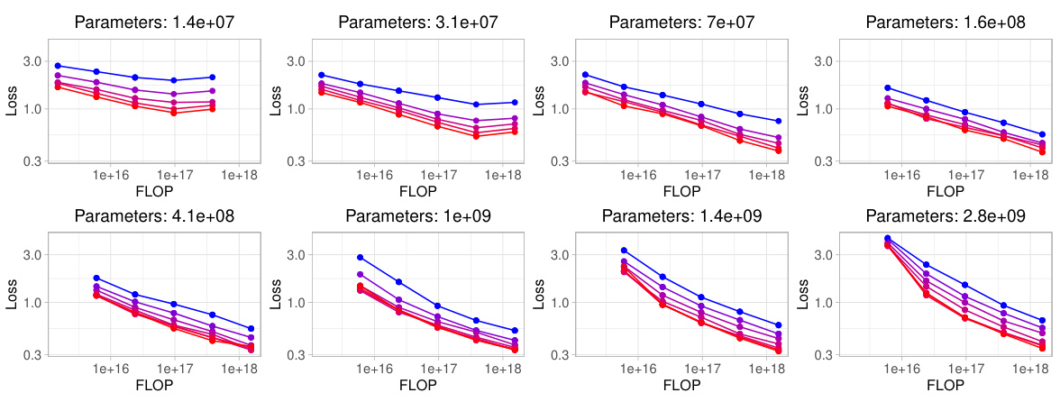
🔼 This figure shows the results of an experiment comparing four different fine-tuning methods for creating text embedding models at various computational budgets. The x-axis represents the computational budget (in FLOPs), and the y-axis represents the contrastive loss achieved. Each method is represented by a different colored line, showing how the loss decreases as the budget increases. The black line shows the optimal loss achievable at each budget (the ‘optimal frontier’), which serves as a benchmark for comparing the methods. This allows one to determine which method is most compute-efficient for a given budget.
read the caption
Figure 1: The optimal loss achieved using four different fine-tuning methods (full fine-tuning, only tuning the bias, low-rank adaptation, and freezing transformer blocks) at given budgets. The horizontal axis is the computational budget in floating point operations (FLOP) and the vertical axis is the contrastive loss. The X marks are datapoints and dotted lines are fitted linear trends for different methods. The solid black line is the 'optimal frontier,' i.e., the optimal loss achievable with a fixed budget and the best method.
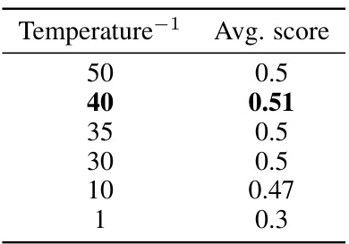
🔼 This table presents the average scores obtained for different temperature values during the grid search for partial tuning. The temperature parameter is inversely proportional to the temperature used for calculating the contrastive loss, which directly impacts the quality of the embeddings produced. The results indicate that a temperature inverse of 40 yields the best performance, suggesting an optimal balance between the positive and negative pairs during the contrastive learning process.
read the caption
Table 1: A comparison of different temperature values
In-depth insights#
Compute-Optimal Tuning#
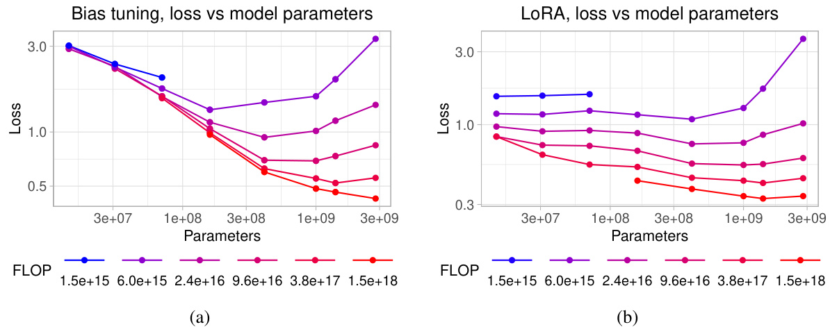
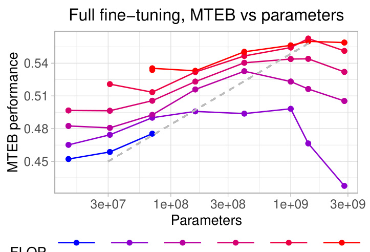
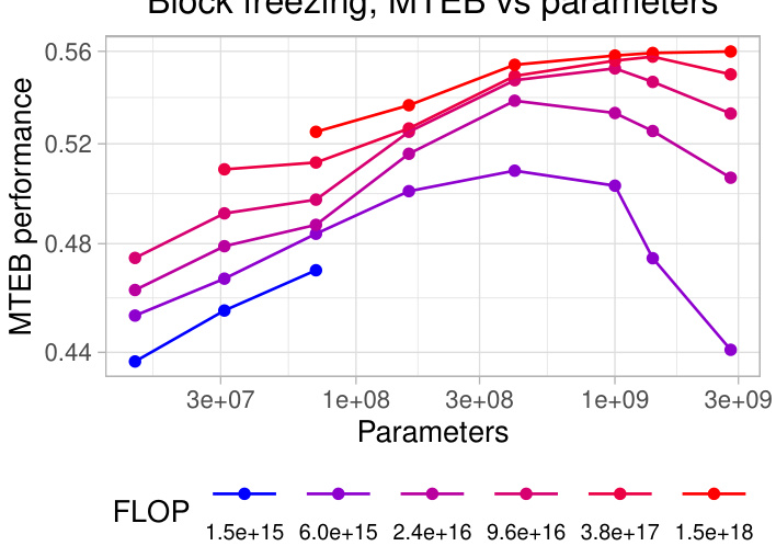
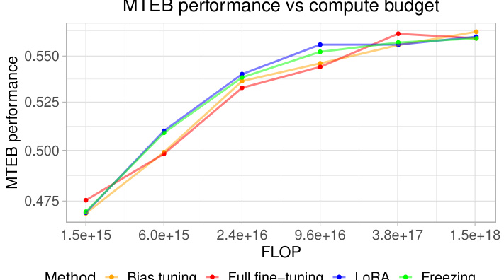
Compute-optimal tuning in the context of language model embeddings focuses on finding the most efficient training configuration given a fixed computational budget. The core idea is to optimize the trade-off between model size, training data size, and fine-tuning method to achieve the best embedding quality while minimizing resource consumption. This involves systematically exploring different configurations (e.g., varying model sizes, datasets, and using methods like full fine-tuning, low-rank adaptation, or bias tuning) and assessing their performance. Key findings often include scaling laws that help predict optimal configurations based on the budget and insights into the relative effectiveness of different fine-tuning techniques at various computational scales. A major contribution is usually an algorithm or recipe that practitioners can use to select the best combination for their specific needs and constraints. The research often demonstrates that simpler methods like low-rank adaptation are superior at higher computational budgets, and that full fine-tuning is preferred at lower budgets. The impact lies in making high-quality language models accessible to users with limited computational resources.
Scaling Laws Analysis#
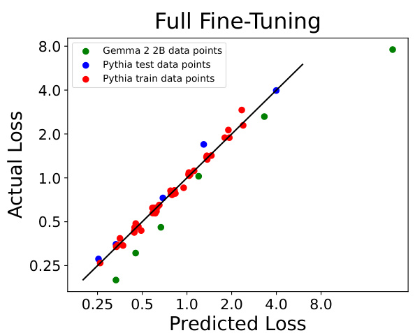
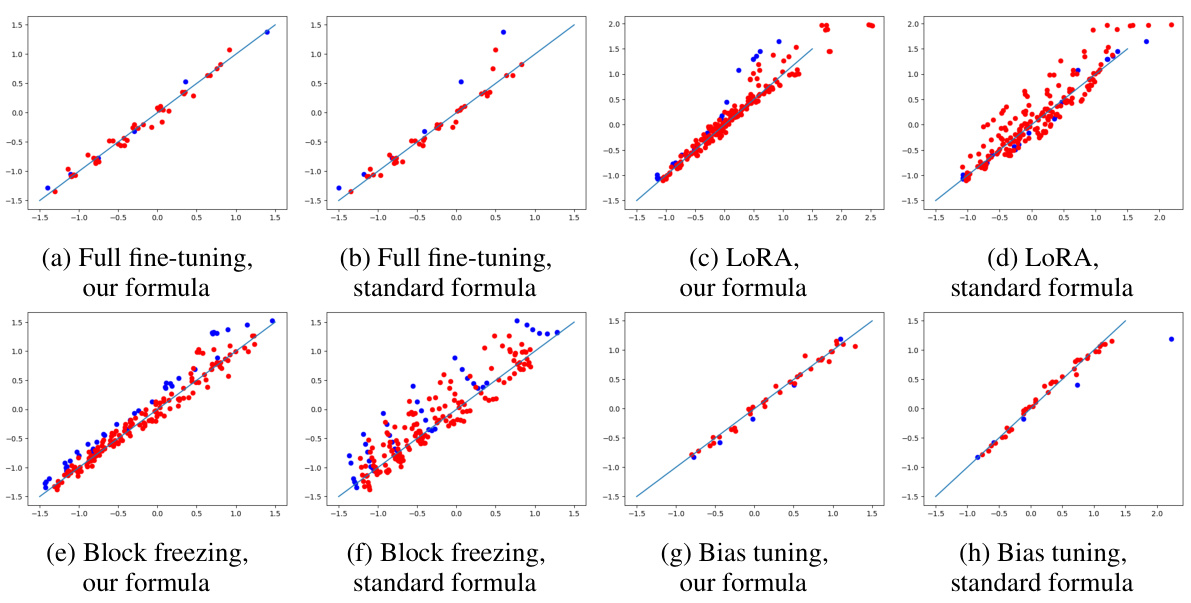
A scaling laws analysis in a text embedding model research paper would likely explore the relationships between model performance (e.g., downstream task accuracy), computational resources (e.g., FLOPs), and dataset size. The analysis might involve fitting empirical models to experimental data, potentially revealing power-law relationships. Key findings could include optimal model sizes for various computational budgets, and the impact of data quantity on performance gains at different model sizes. The analysis might identify regions where parameter-efficient fine-tuning methods become advantageous compared to full fine-tuning, particularly when computational resources are scarce. The research could also assess the generalizability of scaling laws across different model architectures, datasets, and fine-tuning strategies, highlighting limitations and areas where additional research is needed. Overall, a thorough scaling laws analysis provides valuable insights into efficient model development, allowing researchers to optimize resource allocation and achieve superior performance.
PEFT Method Effects#
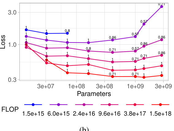
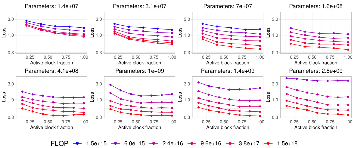
Analyzing the effects of Parameter-Efficient Fine-Tuning (PEFT) methods on the performance of text embedding models reveals crucial insights into optimizing resource utilization. Full fine-tuning, while offering superior performance, is computationally expensive. PEFT methods, like LoRA and block freezing, provide a compelling alternative by significantly reducing the number of updated parameters. LoRA, in particular, shows promise by achieving a good balance between performance and efficiency, with optimal rank selection crucial. Block freezing offers a straightforward technique where freezing blocks at the beginning of the Transformer architecture trades off some accuracy for computational savings. The choice of the best PEFT method heavily depends on the available computational budget. For higher budgets, full fine-tuning might be preferable, while for lower budgets, LoRA or block freezing become more attractive. Further research should investigate the interplay between model architecture, dataset characteristics, and PEFT hyperparameters to establish more robust guidelines for selecting the most appropriate technique.
Benchmark Evaluation#
A robust benchmark evaluation is crucial for assessing the effectiveness of text embedding models. It should involve a diverse range of tasks, encompassing diverse aspects of semantic understanding, such as semantic similarity, document retrieval, and clustering. The evaluation needs to be comprehensive, considering various dataset sizes and complexities. Quantitative metrics should be carefully selected and reported to enable a fair comparison across different models. Furthermore, the evaluation process must be transparent and reproducible, clearly specifying the datasets, evaluation protocols, and metrics used. This allows other researchers to replicate the results and ensure the validity and generalizability of the findings. Finally, a critical analysis of the strengths and weaknesses of different models across tasks is vital for a thorough evaluation, providing insights that go beyond mere performance numbers.
Future Research#
Future research directions stemming from this compute-optimal embedding model study could explore several avenues. Extending the scaling laws to a broader range of language models beyond the Pythia family is crucial to establish generalizability. Investigating the impact of different data distributions and fine-tuning objectives on the scaling laws would enhance the model’s robustness. Exploring alternative architectural designs and parameter-efficient fine-tuning techniques is warranted. Furthermore, analyzing the trade-offs between computational cost, embedding quality, and downstream task performance is crucial for practical applications. A more in-depth examination of the data-constrained regime is necessary, as well as understanding the interaction between model size, data quantity, and compute constraints in that scenario. Finally, incorporating hard negative sampling and exploring other embedding extraction methods to further improve the accuracy and efficiency of embeddings would be valuable future work.
More visual insights#
More on figures
🔼 This figure shows the optimal contrastive loss achievable across four different fine-tuning methods: full fine-tuning, bias-only tuning, low-rank adaptation (LoRA), and block freezing. The x-axis represents the computational budget (in FLOPs), and the y-axis represents the contrastive loss. Each method’s performance is plotted, along with a fitted linear trend. The solid black line indicates the optimal loss achievable for any given budget, representing the optimal frontier across all four methods. This allows for easy comparison of the methods’ compute-efficiency in achieving minimal loss.
read the caption
Figure 1: The optimal loss achieved using four different fine-tuning methods (full fine-tuning, only tuning the bias, low-rank adaptation, and freezing transformer blocks) at given budgets. The horizontal axis is the computational budget in floating point operations (FLOP) and the vertical axis is the contrastive loss. The X marks are datapoints and dotted lines are fitted linear trends for different methods. The solid black line is the 'optimal frontier,' i.e., the optimal loss achievable with a fixed budget and the best method.
🔼 This figure illustrates the trade-off between computational cost (FLOPs) and the achieved contrastive loss for four different fine-tuning methods: full fine-tuning, bias-only tuning, low-rank adaptation (LoRA), and block freezing. It shows that different methods are optimal at different computational budget levels, with full fine-tuning being best for low budgets and LoRA best for high budgets. The ‘optimal frontier’ line represents the lowest achievable loss for each computational budget, regardless of the fine-tuning method used.
read the caption
Figure 1: The optimal loss achieved using four different fine-tuning methods (full fine-tuning, only tuning the bias, low-rank adaptation, and freezing transformer blocks) at given budgets. The horizontal axis is the computational budget in floating point operations (FLOP) and the vertical axis is the contrastive loss. The X marks are datapoints and dotted lines are fitted linear trends for different methods. The solid black line is the 'optimal frontier,' i.e., the optimal loss achievable with a fixed budget and the best method.
🔼 This figure shows the relationship between computational budget (in FLOPs) and the achieved contrastive loss for four different fine-tuning methods: full fine-tuning, bias tuning, low-rank adaptation (LoRA), and block freezing. The optimal loss for each method is plotted, revealing a trade-off between computational cost and model performance. A ‘optimal frontier’ line is also presented, indicating the best achievable loss for a given budget across all methods.
read the caption
Figure 1: The optimal loss achieved using four different fine-tuning methods (full fine-tuning, only tuning the bias, low-rank adaptation, and freezing transformer blocks) at given budgets. The horizontal axis is the computational budget in floating point operations (FLOP) and the vertical axis is the contrastive loss. The X marks are datapoints and dotted lines are fitted linear trends for different methods. The solid black line is the 'optimal frontier,' i.e., the optimal loss achievable with a fixed budget and the best method.
🔼 This figure shows the optimal contrastive loss achieved at different computational budgets using four different fine-tuning methods: full fine-tuning, bias tuning, low-rank adaptation (LoRA), and block freezing. The x-axis represents the computational budget (in FLOPs), and the y-axis represents the contrastive loss. The optimal loss for each method is plotted, along with a fitted linear trend. The black line represents the optimal frontier, indicating the lowest achievable loss for a given computational budget across all methods.
read the caption
Figure 1: The optimal loss achieved using four different fine-tuning methods (full fine-tuning, only tuning the bias, low-rank adaptation, and freezing transformer blocks) at given budgets. The horizontal axis is the computational budget in floating point operations (FLOP) and the vertical axis is the contrastive loss. The X marks are datapoints and dotted lines are fitted linear trends for different methods. The solid black line is the 'optimal frontier,' i.e., the optimal loss achievable with a fixed budget and the best method.

🔼 This figure illustrates the trade-off between computational budget (measured in FLOPs) and the achieved contrastive loss for four different fine-tuning methods. The optimal frontier line shows the lowest loss achievable at each budget level by selecting the best method. It demonstrates that different methods are optimal at different budget ranges, with full fine-tuning being best at low budgets and low-rank adaptation best at high budgets.
read the caption
Figure 1: The optimal loss achieved using four different fine-tuning methods (full fine-tuning, only tuning the bias, low-rank adaptation, and freezing transformer blocks) at given budgets. The horizontal axis is the computational budget in floating point operations (FLOP) and the vertical axis is the contrastive loss. The X marks are datapoints and dotted lines are fitted linear trends for different methods. The solid black line is the 'optimal frontier,' i.e., the optimal loss achievable with a fixed budget and the best method.

🔼 This figure shows the trade-off between computational cost (FLOPs) and the achieved contrastive loss for four different fine-tuning methods: full fine-tuning, bias-only tuning, low-rank adaptation (LoRA), and block freezing. The optimal frontier line indicates the lowest achievable loss for each computational budget, showing which fine-tuning method performs best at different resource levels. The plot helps to determine a compute-optimal recipe for training text embedding models.
read the caption
Figure 1: The optimal loss achieved using four different fine-tuning methods (full fine-tuning, only tuning the bias, low-rank adaptation, and freezing transformer blocks) at given budgets. The horizontal axis is the computational budget in floating point operations (FLOP) and the vertical axis is the contrastive loss. The X marks are datapoints and dotted lines are fitted linear trends for different methods. The solid black line is the 'optimal frontier,' i.e., the optimal loss achievable with a fixed budget and the best method.

🔼 This figure illustrates the trade-off between computational budget (FLOPs) and achieved contrastive loss for four different fine-tuning methods: full fine-tuning, bias-only tuning, low-rank adaptation (LoRA), and block freezing. The optimal frontier line shows the lowest achievable loss for each budget, highlighting the most compute-efficient method for a given budget. The results indicate that full fine-tuning is optimal at lower budgets and LoRA at higher budgets.
read the caption
Figure 1: The optimal loss achieved using four different fine-tuning methods (full fine-tuning, only tuning the bias, low-rank adaptation, and freezing transformer blocks) at given budgets. The horizontal axis is the computational budget in floating point operations (FLOP) and the vertical axis is the contrastive loss. The X marks are datapoints and dotted lines are fitted linear trends for different methods. The solid black line is the 'optimal frontier,' i.e., the optimal loss achievable with a fixed budget and the best method.
🔼 This figure shows the relationship between computational budget (in FLOPs) and the achieved contrastive loss for four different fine-tuning methods. Each method is represented by a different colored line with data points indicating experimental results. A fitted trendline shows the best achievable loss for a given budget, regardless of the method used, and represents the optimal frontier. The figure suggests that different fine-tuning methods are optimal at different budget levels.
read the caption
Figure 1: The optimal loss achieved using four different fine-tuning methods (full fine-tuning, only tuning the bias, low-rank adaptation, and freezing transformer blocks) at given budgets. The horizontal axis is the computational budget in floating point operations (FLOP) and the vertical axis is the contrastive loss. The X marks are datapoints and dotted lines are fitted linear trends for different methods. The solid black line is the 'optimal frontier,' i.e., the optimal loss achievable with a fixed budget and the best method.
🔼 This figure shows the optimal contrastive loss achieved by four different fine-tuning methods at various computational budgets. The x-axis represents the computational budget (in FLOPs), and the y-axis represents the contrastive loss. Each method’s performance is shown with data points and a fitted trendline. A black line shows the optimal loss achievable at each budget across all methods, forming an ‘optimal frontier’. The methods compared are full fine-tuning, bias tuning, low-rank adaptation (LoRA), and block freezing.
read the caption
Figure 1: The optimal loss achieved using four different fine-tuning methods (full fine-tuning, only tuning the bias, low-rank adaptation, and freezing transformer blocks) at given budgets. The horizontal axis is the computational budget in floating point operations (FLOP) and the vertical axis is the contrastive loss. The X marks are datapoints and dotted lines are fitted linear trends for different methods. The solid black line is the 'optimal frontier,' i.e., the optimal loss achievable with a fixed budget and the best method.

🔼 This figure shows the optimal contrastive loss achieved by four different fine-tuning methods across various computational budgets. The x-axis represents the computational budget (in FLOPs), and the y-axis represents the contrastive loss. The optimal frontier line indicates the lowest achievable loss for each budget, showing that different methods are optimal at different budget levels. The figure demonstrates the trade-off between computational cost and model performance.
read the caption
Figure 1: The optimal loss achieved using four different fine-tuning methods (full fine-tuning, only tuning the bias, low-rank adaptation, and freezing transformer blocks) at given budgets. The horizontal axis is the computational budget in floating point operations (FLOP) and the vertical axis is the contrastive loss. The X marks are datapoints and dotted lines are fitted linear trends for different methods. The solid black line is the 'optimal frontier,' i.e., the optimal loss achievable with a fixed budget and the best method.

🔼 This figure shows the trade-off between computational budget (in FLOPs) and the achieved contrastive loss for four different fine-tuning methods: full fine-tuning, bias-only tuning, low-rank adaptation (LoRA), and block freezing. The optimal loss for each method is plotted, and a line representing the optimal frontier (lowest loss for each budget) is shown. The figure illustrates the compute-optimal recipe: for lower budgets, full fine-tuning is best; for higher budgets, LoRA is superior.
read the caption
Figure 1: The optimal loss achieved using four different fine-tuning methods (full fine-tuning, only tuning the bias, low-rank adaptation, and freezing transformer blocks) at given budgets. The horizontal axis is the computational budget in floating point operations (FLOP) and the vertical axis is the contrastive loss. The X marks are datapoints and dotted lines are fitted linear trends for different methods. The solid black line is the 'optimal frontier,' i.e., the optimal loss achievable with a fixed budget and the best method.
🔼 This figure shows the trade-off between computational cost (FLOPs) and the achieved contrastive loss for four different fine-tuning methods: full fine-tuning, bias-only tuning, low-rank adaptation (LoRA), and block freezing. The optimal frontier line indicates the lowest achievable loss for each computational budget, showing which method is most compute-efficient for a given budget. The plot demonstrates that different methods are optimal at different budget levels, with full fine-tuning performing best at lower budgets and LoRA being more effective at higher budgets.
read the caption
Figure 1: The optimal loss achieved using four different fine-tuning methods (full fine-tuning, only tuning the bias, low-rank adaptation, and freezing transformer blocks) at given budgets. The horizontal axis is the computational budget in floating point operations (FLOP) and the vertical axis is the contrastive loss. The X marks are datapoints and dotted lines are fitted linear trends for different methods. The solid black line is the 'optimal frontier,' i.e., the optimal loss achievable with a fixed budget and the best method.

🔼 This figure illustrates the trade-off between computational cost (FLOPs) and the achieved contrastive loss for four different text embedding fine-tuning methods. It shows that different methods are optimal at different computational budgets. The ‘optimal frontier’ line represents the lowest achievable loss for each budget, indicating the best method to use given resource constraints.
read the caption
Figure 1: The optimal loss achieved using four different fine-tuning methods (full fine-tuning, only tuning the bias, low-rank adaptation, and freezing transformer blocks) at given budgets. The horizontal axis is the computational budget in floating point operations (FLOP) and the vertical axis is the contrastive loss. The X marks are datapoints and dotted lines are fitted linear trends for different methods. The solid black line is the 'optimal frontier,' i.e., the optimal loss achievable with a fixed budget and the best method.
🔼 This figure shows the trade-off between computational cost and achieved contrastive loss for four different fine-tuning methods: full fine-tuning, bias-only tuning, low-rank adaptation (LoRA), and block freezing. The optimal frontier line indicates the lowest loss achievable for a given computational budget, selecting the best method at each budget. The figure highlights that different methods are optimal at different budget levels, suggesting a strategy for choosing the most compute-efficient method for any given budget.
read the caption
Figure 1: The optimal loss achieved using four different fine-tuning methods (full fine-tuning, only tuning the bias, low-rank adaptation, and freezing transformer blocks) at given budgets. The horizontal axis is the computational budget in floating point operations (FLOP) and the vertical axis is the contrastive loss. The X marks are datapoints and dotted lines are fitted linear trends for different methods. The solid black line is the 'optimal frontier,' i.e., the optimal loss achievable with a fixed budget and the best method.

🔼 This figure shows the optimal contrastive loss achieved for four different fine-tuning methods across various computational budgets. The x-axis represents the computational budget (in FLOPs), and the y-axis shows the contrastive loss. Each method’s performance is plotted, with a fitted line showing its trend. The black line represents the ‘optimal frontier,’ indicating the lowest achievable loss for each budget using the best-performing method among the four.
read the caption
Figure 1: The optimal loss achieved using four different fine-tuning methods (full fine-tuning, only tuning the bias, low-rank adaptation, and freezing transformer blocks) at given budgets. The horizontal axis is the computational budget in floating point operations (FLOP) and the vertical axis is the contrastive loss. The X marks are datapoints and dotted lines are fitted linear trends for different methods. The solid black line is the 'optimal frontier,' i.e., the optimal loss achievable with a fixed budget and the best method.

🔼 This figure illustrates the trade-off between computational budget (in FLOPs) and the achieved contrastive loss for four different fine-tuning methods. Each method (full fine-tuning, bias-only tuning, low-rank adaptation (LoRA), and block freezing) is represented by a series of data points, each corresponding to a different model size and training data. The dotted lines show linear fits to the data points for each method. The black line represents the optimal frontier, indicating the lowest achievable loss for any given computational budget, regardless of the fine-tuning method used. The figure demonstrates that different fine-tuning methods are optimal at different budget levels.
read the caption
Figure 1: The optimal loss achieved using four different fine-tuning methods (full fine-tuning, only tuning the bias, low-rank adaptation, and freezing transformer blocks) at given budgets. The horizontal axis is the computational budget in floating point operations (FLOP) and the vertical axis is the contrastive loss. The X marks are datapoints and dotted lines are fitted linear trends for different methods. The solid black line is the 'optimal frontier,' i.e., the optimal loss achievable with a fixed budget and the best method.

🔼 This figure shows the trade-off between computational cost and model performance (contrastive loss) for four different fine-tuning methods. The optimal frontier line represents the lowest achievable loss for each computational budget. The plot reveals that different fine-tuning methods are optimal at different budget levels, suggesting a compute-optimal recipe exists.
read the caption
Figure 1: The optimal loss achieved using four different fine-tuning methods (full fine-tuning, only tuning the bias, low-rank adaptation, and freezing transformer blocks) at given budgets. The horizontal axis is the computational budget in floating point operations (FLOP) and the vertical axis is the contrastive loss. The X marks are datapoints and dotted lines are fitted linear trends for different methods. The solid black line is the 'optimal frontier,' i.e., the optimal loss achievable with a fixed budget and the best method.

🔼 This figure shows the relationship between computational budget (in FLOPs) and the achieved contrastive loss for four different fine-tuning methods: full fine-tuning, bias-only tuning, low-rank adaptation (LoRA), and block freezing. The optimal loss for each method is plotted, revealing an optimal frontier that represents the lowest achievable loss for a given computational budget. The X marks represent experimental data points, and the dotted lines represent fitted linear trends. The solid black line represents the overall optimal frontier, indicating the best loss achievable for any given budget by selecting the best method among the four.
read the caption
Figure 1: The optimal loss achieved using four different fine-tuning methods (full fine-tuning, only tuning the bias, low-rank adaptation, and freezing transformer blocks) at given budgets. The horizontal axis is the computational budget in floating point operations (FLOP) and the vertical axis is the contrastive loss. The X marks are datapoints and dotted lines are fitted linear trends for different methods. The solid black line is the 'optimal frontier,' i.e., the optimal loss achievable with a fixed budget and the best method.
🔼 This figure shows the relationship between computational budget (in FLOPs) and the achieved contrastive loss for four different fine-tuning methods: full fine-tuning, bias-only tuning, low-rank adaptation (LoRA), and block freezing. The optimal frontier line represents the lowest achievable loss for a given computational budget, showing which method is most efficient at different resource levels.
read the caption
Figure 1: The optimal loss achieved using four different fine-tuning methods (full fine-tuning, only tuning the bias, low-rank adaptation, and freezing transformer blocks) at given budgets. The horizontal axis is the computational budget in floating point operations (FLOP) and the vertical axis is the contrastive loss. The X marks are datapoints and dotted lines are fitted linear trends for different methods. The solid black line is the 'optimal frontier,' i.e., the optimal loss achievable with a fixed budget and the best method.

🔼 This figure shows the relationship between computational budget (in FLOPs) and the contrastive loss achieved by four different fine-tuning methods: full fine-tuning, bias-only tuning, low-rank adaptation (LoRA), and block freezing. The optimal loss for each method is plotted, revealing the trade-offs between computational cost and model performance. The ‘optimal frontier’ line represents the lowest achievable loss for a given budget, indicating the best method to use at each budget level.
read the caption
Figure 1: The optimal loss achieved using four different fine-tuning methods (full fine-tuning, only tuning the bias, low-rank adaptation, and freezing transformer blocks) at given budgets. The horizontal axis is the computational budget in floating point operations (FLOP) and the vertical axis is the contrastive loss. The X marks are datapoints and dotted lines are fitted linear trends for different methods. The solid black line is the 'optimal frontier,' i.e., the optimal loss achievable with a fixed budget and the best method.
🔼 This figure shows the results of an experiment comparing four different fine-tuning methods for creating text embedding models: full fine-tuning, bias-only tuning, low-rank adaptation (LoRA), and block freezing. The x-axis represents the computational budget (in FLOPs), and the y-axis represents the contrastive loss achieved by each method. Data points are plotted, and linear trends are fitted for each method. A solid black line indicates the ‘optimal frontier,’ representing the lowest achievable loss for any given computational budget, achieved by selecting the best method at each budget.
read the caption
Figure 1: The optimal loss achieved using four different fine-tuning methods (full fine-tuning, only tuning the bias, low-rank adaptation, and freezing transformer blocks) at given budgets. The horizontal axis is the computational budget in floating point operations (FLOP) and the vertical axis is the contrastive loss. The X marks are datapoints and dotted lines are fitted linear trends for different methods. The solid black line is the 'optimal frontier,' i.e., the optimal loss achievable with a fixed budget and the best method.

🔼 This figure shows the trade-off between computational cost and model performance (contrastive loss) for four different fine-tuning methods. The x-axis represents the computational budget (in FLOPs), and the y-axis shows the achieved contrastive loss. Each method’s performance is represented by a line, showing how loss decreases with increased computational budget. The optimal frontier line indicates the lowest achievable loss for a given budget, which may be achieved by different methods at different budgets.
read the caption
Figure 1: The optimal loss achieved using four different fine-tuning methods (full fine-tuning, only tuning the bias, low-rank adaptation, and freezing transformer blocks) at given budgets. The horizontal axis is the computational budget in floating point operations (FLOP) and the vertical axis is the contrastive loss. The X marks are datapoints and dotted lines are fitted linear trends for different methods. The solid black line is the 'optimal frontier,' i.e., the optimal loss achievable with a fixed budget and the best method.

🔼 This figure shows the trade-off between computational budget (in FLOPs) and the achieved contrastive loss for four different fine-tuning methods. It reveals that different fine-tuning strategies are optimal at different computational budget levels. The ‘optimal frontier’ line represents the lowest achievable loss for each budget, indicating the best-performing method for a given computational constraint.
read the caption
Figure 1: The optimal loss achieved using four different fine-tuning methods (full fine-tuning, only tuning the bias, low-rank adaptation, and freezing transformer blocks) at given budgets. The horizontal axis is the computational budget in floating point operations (FLOP) and the vertical axis is the contrastive loss. The X marks are datapoints and dotted lines are fitted linear trends for different methods. The solid black line is the 'optimal frontier,' i.e., the optimal loss achievable with a fixed budget and the best method.
More on tables

🔼 This table presents a comparison of the average scores obtained using two different pooling methods: mean pooling and last pooling. The results show that mean pooling achieves a higher average score (0.47) compared to last pooling (0.36), indicating that mean pooling is a more effective method for this task.
read the caption
Table 2: Mean pooling works better than last pooling.

🔼 This table presents the results of a hyperparameter search for the learning rate used in LoRA fine-tuning. Three different LoRA ranks (8, 16, and 32) were tested, each with three different learning rates (1e2, 1e3, and 1e4). The loss achieved for each combination of LoRA rank and learning rate is shown. The table helps in determining the optimal learning rate for different LoRA ranks.
read the caption
Table 3: Learning rate for LoRA.
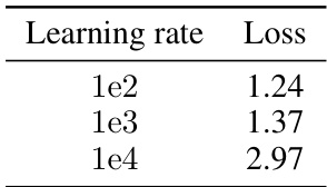
🔼 This table shows the average score achieved on a subset of MTEB benchmark for different temperature values used during the training of embedding models with partial tuning. The best score is 0.51, achieved with temperature = 40.
read the caption
Table 1: A comparison of different temperature values
Full paper#

