↗ OpenReview ↗ NeurIPS Homepage ↗ Chat
TL;DR#
Many real-world problems involve optimizing functions defined on node subsets within graphs (e.g., influence maximization, network resilience). However, traditional optimization techniques often struggle due to the combinatorial explosion of the search space and the high cost of evaluating the objective function. This frequently limits their effectiveness and scalability. The paper addresses these limitations by introducing GraphComBO, a novel framework that leverages the sample efficiency of Bayesian Optimization.
GraphComBO maps the node subset optimization problem onto a new combinatorial graph, cleverly navigating this space via a recursive algorithm that samples local subgraphs. This local modeling approach reduces computational complexity. A Gaussian Process surrogate model captures the function’s behavior effectively, and an acquisition function guides the selection of the next node subset to evaluate. Extensive experiments show that GraphComBO substantially outperforms existing approaches in both synthetic and real-world settings, establishing it as a powerful tool for various graph optimization tasks.
Key Takeaways#
Why does it matter?#
This paper is important because it presents a novel Bayesian optimization framework for efficiently optimizing black-box functions over node subsets in graphs. This is a significant advancement as traditional methods are often computationally expensive or limited to specific tasks. The proposed framework’s versatility and efficiency make it highly relevant to various fields like network science, social network analysis, and epidemiology where optimizing over node subsets is crucial. It also opens up new avenues for research into sample-efficient black-box optimization techniques within complex graph structures.
Visual Insights#

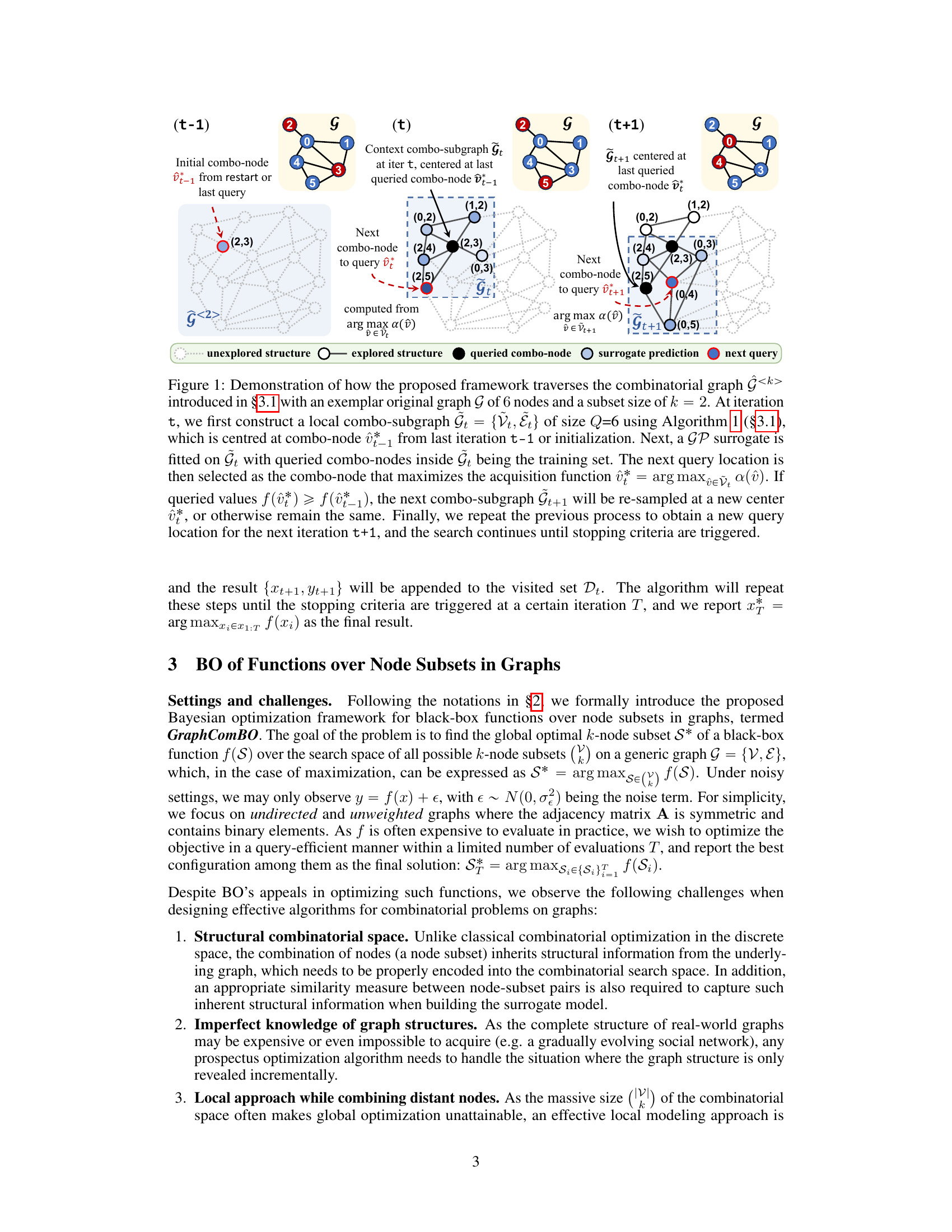
This figure illustrates the process of the proposed framework traversing a combinatorial graph. It shows how a local combo-subgraph is constructed, a Gaussian Process (GP) surrogate model is fitted, and the acquisition function is used to select the next node to query. The process iteratively refines the search until a stopping criterion is met.

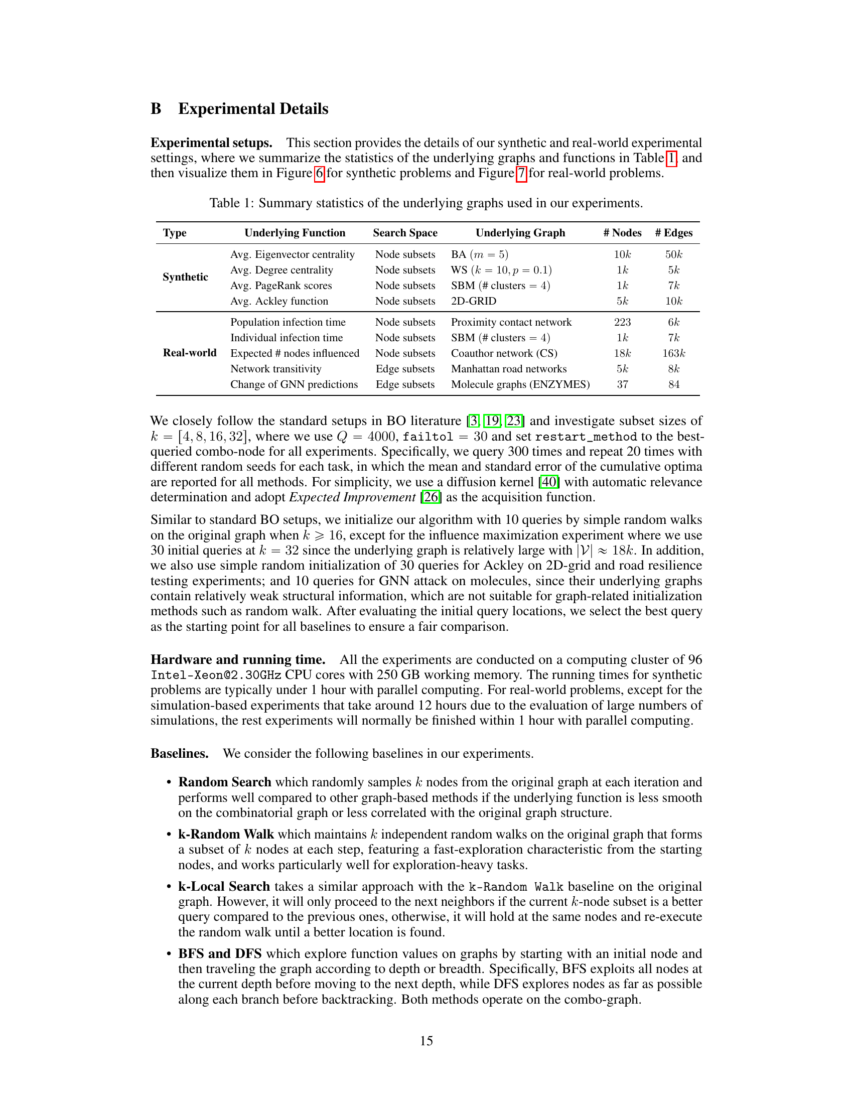
This table summarizes the characteristics of the graphs used in the experiments presented in the paper. For each graph, it lists the type (synthetic or real-world), the underlying function optimized on that graph, the search space (node subsets or edge subsets), the specific type of graph (e.g., Barabási-Albert, Watts-Strogatz, Stochastic Block Model, etc.), and the number of nodes and edges in the graph.
In-depth insights#
GraphComBO Framework#
The GraphComBO framework presents a novel approach to Bayesian Optimization (BO) for tackling complex combinatorial optimization problems within graph structures. Its core innovation lies in transforming the original graph into a ‘combo-graph,’ where nodes represent k-node subsets and edges connect subsets differing by only one node. This clever mapping allows BO to efficiently explore the vast search space, even with potentially large or partially unknown graphs. A recursive algorithm then samples local combo-subgraphs, enabling a sample-efficient, function-agnostic optimization process. GraphComBO’s local modeling approach cleverly balances exploration and exploitation, handling the challenges of expensive function evaluations and the inherent structural complexity of graph data. The framework’s effectiveness is demonstrated through comprehensive experiments on diverse graph types, showcasing its superiority to traditional methods in handling various optimization tasks. The key strength is its versatility, applying to scenarios where the graph structure is not fully known and the objective function is a black box.
Combo-graph Traversal#
The concept of “Combo-graph Traversal” presents a novel approach to navigating the vast search space inherent in combinatorial optimization problems on graphs. Instead of directly searching the space of all possible k-node subsets, which is computationally prohibitive, the method constructs a “combo-graph” where each node represents a k-node subset. Efficient traversal is crucial, and this is achieved through a recursive algorithm that progressively samples local combo-subgraphs. This local modeling strategy is key to scalability, as it avoids the need for global modeling of the enormous combo-graph. The recursive algorithm smartly balances exploration and exploitation, ensuring the algorithm does not get stuck in local optima while also efficiently using the available evaluations of the expensive black-box function being optimized. The recursive nature allows it to adapt to partially revealed graph structures, making it robust to real-world scenarios with incomplete information. The combination of the combo-graph representation and the recursive sampling strategy is the core innovation of the approach, offering a powerful and scalable way to tackle complex combinatorial graph optimization problems.
Surrogate Model Choice#
Surrogate model selection is crucial for Bayesian Optimization’s (BO) effectiveness. The choice significantly impacts BO’s ability to balance exploration and exploitation, directly affecting the efficiency and accuracy of the global optimum search. Gaussian Processes (GPs) are frequently used due to their ability to quantify uncertainty, but their computational cost scales cubically with the number of observations, limiting scalability. Therefore, considerations must be made regarding computational constraints and the nature of the objective function. If the objective function is smooth, simpler models might suffice, reducing computational overhead. Conversely, for complex functions exhibiting high dimensionality and non-linearity, a more powerful and computationally expensive model like a GP might be necessary. Local modeling techniques, which focus on a smaller region of the search space, offer a compromise. They reduce computational demand while preserving accuracy, particularly when dealing with large search spaces. The choice of kernel within the GP also matters, as it dictates how similarity between data points is measured. Careful selection is needed to capture the underlying structure of the objective function. Finally, the choice of surrogate model isn’t isolated; it interacts with acquisition functions and the sampling strategy. A holistic approach, integrating model complexity, computational resources, and objective function characteristics, is essential for optimal surrogate model selection in BO.
Scalability and Noise#
The scalability of Bayesian Optimization (BO) methods for large-scale problems, especially those involving graphs, is a critical concern. The computational cost of BO often scales poorly with the size of the search space. GraphComBO addresses this by employing a local modeling approach, focusing on a smaller subgraph of the combinatorial graph at each iteration, rather than attempting global optimization. This significantly reduces the computational burden, enabling BO to be applied to larger graphs. Furthermore, real-world datasets often contain noisy observations, which can negatively impact the performance of BO. GraphComBO’s robustness to noise is demonstrated through experiments with various noise levels, showing it maintains reasonable performance even with significant amounts of noise. The impact of hyperparameters like subgraph size on both scalability and noise resilience is also analyzed. A balance must be struck between exploration and exploitation, with larger subgraphs improving exploration but increasing computational cost, while a smaller subgraph increases efficiency but might miss promising regions. The choice of acquisition function and kernel also plays a crucial role in handling noise effectively.
Future Research#
The paper’s “Future Research” section could productively explore several avenues. Addressing the limitations of the current approach, particularly concerning scalability with larger k values and the impact of varying signal smoothness, is crucial. Investigating alternative surrogate models beyond Gaussian Processes, perhaps incorporating graph neural networks for more effective handling of graph structure, would enhance robustness. Developing adaptive methods for adjusting hyperparameters like combo-subgraph size (Q) and failure tolerance (failtol) dynamically during the search process would significantly improve performance. Finally, exploring the use of prior information or knowledge about the objective function or the graph structure could drastically reduce the search space and enhance query efficiency, particularly useful for real-world scenarios where obtaining complete graph information might be expensive or impractical.
More visual insights#
More on figures
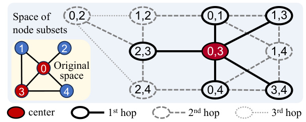
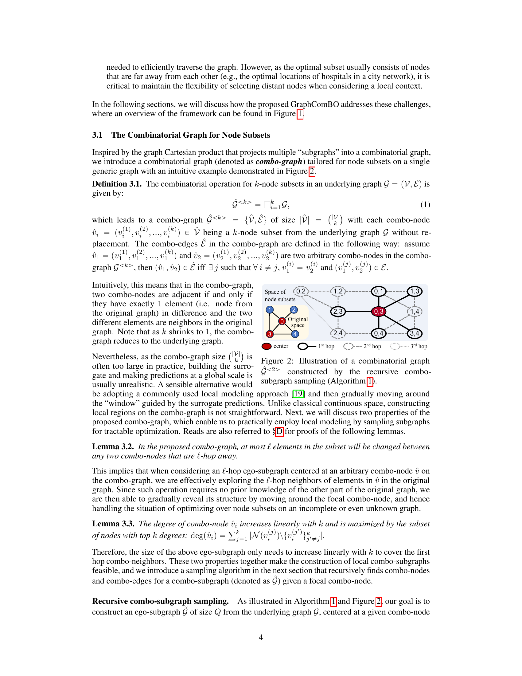
This figure illustrates how the recursive combo-subgraph sampling algorithm constructs a combinatorial graph. The original graph (a small example graph is shown) is transformed into a combinatorial graph where nodes represent k-node subsets (k=2 in this case). Edges connect subsets that differ by only one node, and those nodes must be adjacent in the original graph. The algorithm recursively samples subgraphs, starting from a central combo-node, expanding by hops, until a size limit is reached. Different line styles represent different hops from the central node. This process is central to GraphComBO’s efficient traversal of the large search space.
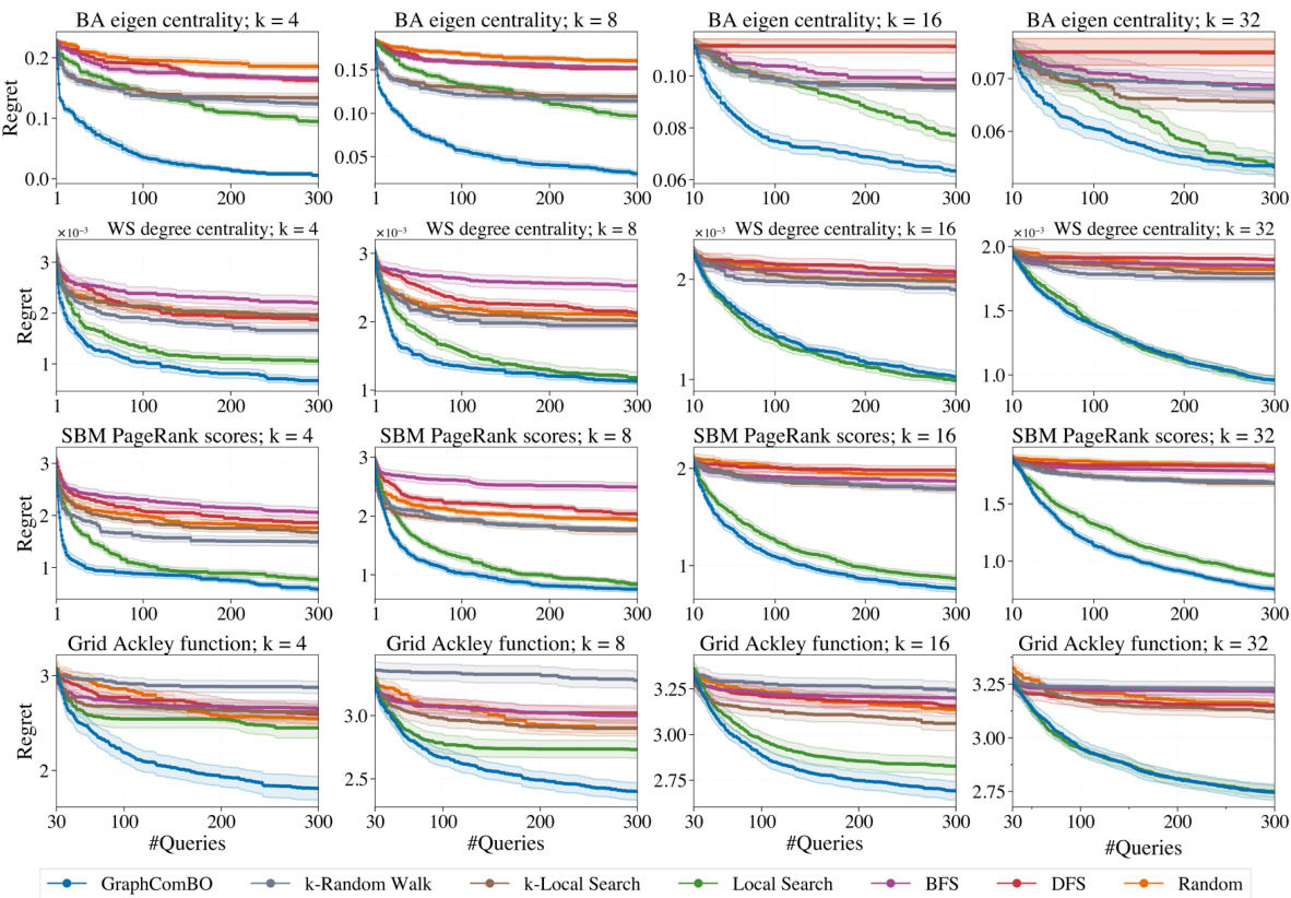
This figure displays the results of four different synthetic experiments on four different types of random graphs (Barabási-Albert, Watts-Strogatz, Stochastic Block Model, and 2D grid). Each experiment aims to find the best subset of k nodes (k=4,8,16,32) that maximizes a specific function (eigen centrality, degree centrality, PageRank scores, and Ackley function). The y-axis represents the ‘Regret’, which is the difference between the optimal value of the objective function and the value found by the algorithm at each iteration. The x-axis shows the number of queries made by the algorithm. Several algorithms (GraphComBO, k-Random Walk, k-Local Search, Local Search, BFS, DFS, and Random) are compared, and their performance is assessed based on the Regret values.
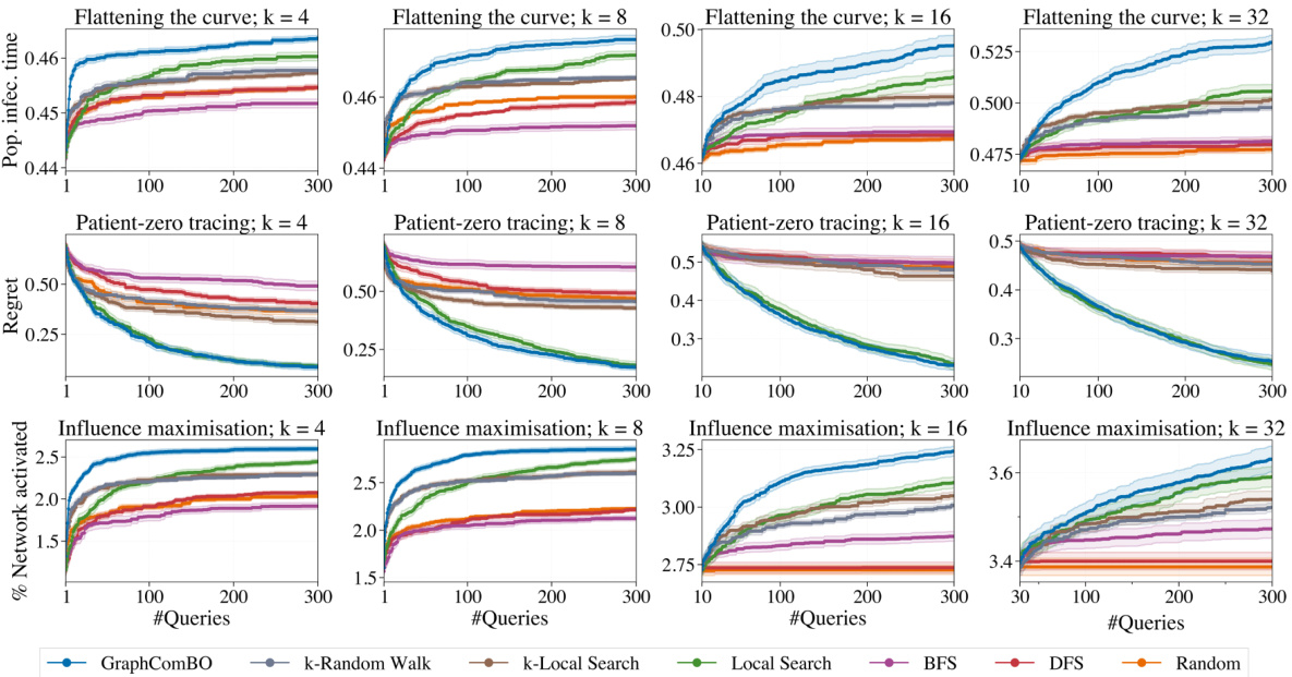
This figure presents the results of four synthetic experiments, each using a different type of random graph (Barabási-Albert, Watts-Strogatz, Stochastic Block Model, and 2D grid) and a different objective function. Each experiment varies the size (k) of the node subsets to be optimized (4, 8, 16, 32). The y-axis shows the regret, which represents the difference between the optimal value found by the algorithm and the actual optimal value. The x-axis represents the number of queries made to the black-box function. The figure compares the performance of GraphComBO against several baseline algorithms (k-Random Walk, BFS, DFS, Random, k-Local Search, Local Search).
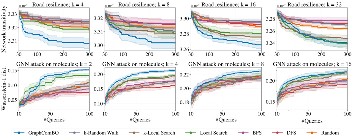
This figure displays the results of experiments on four different types of synthetic graph networks (Barabási-Albert, Watts-Strogatz, Stochastic Block Model, and 2D grid). Each network was tested with four different subset sizes (k = 4, 8, 16, 32). The y-axis shows the regret, which represents the difference between the optimal value found and the true optimal value. The x-axis represents the number of queries made during the optimization process. Different optimization methods were compared: GraphComBO, k-random walk, BFS, DFS, random, k-local search and local search. The results show how the regret decreases over the number of queries for each method and network type, illustrating the effectiveness of the proposed GraphComBO method.

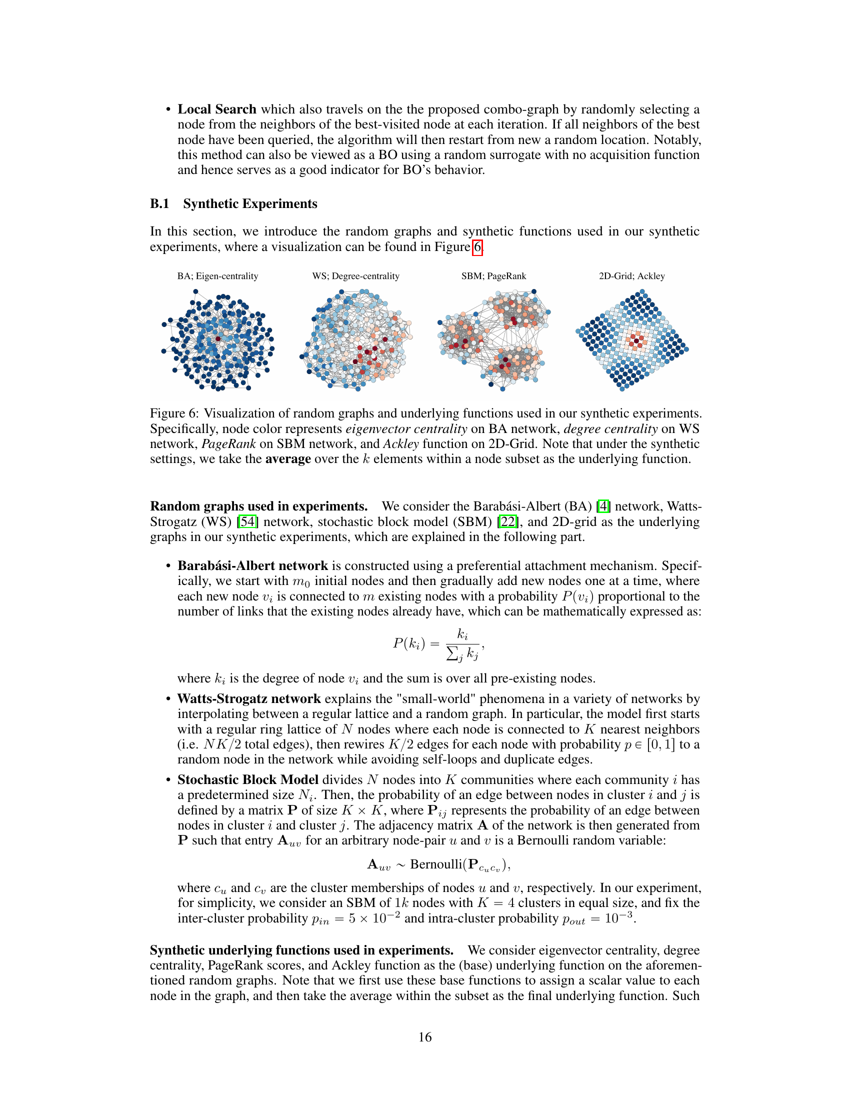
This figure visualizes four different types of random graphs used in the synthetic experiments of the paper: Barabási-Albert (BA), Watts-Strogatz (WS), Stochastic Block Model (SBM), and 2D-grid. Each graph is color-coded to represent the value of a specific function (eigenvector centrality, degree centrality, PageRank, and Ackley function respectively). The color intensity represents the magnitude of the function value at each node. In the synthetic experiments, the average function value over a subset of k nodes is used as the final underlying function for optimization.

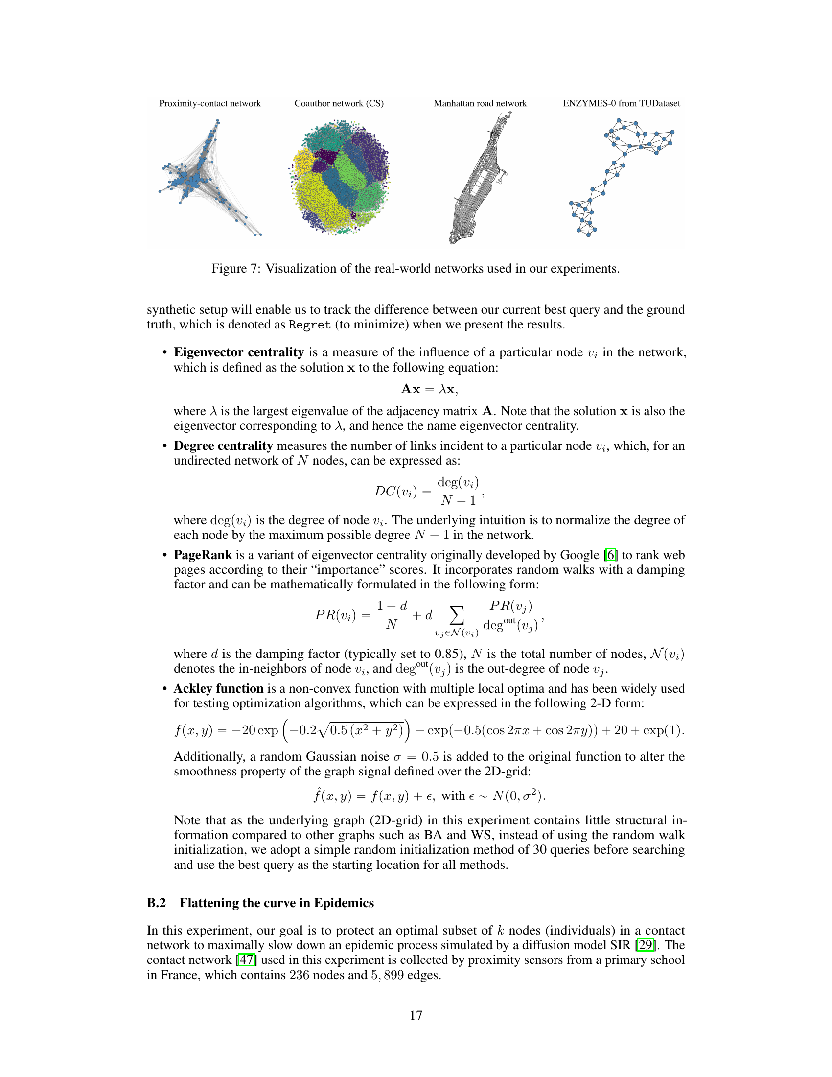
This figure visualizes four real-world networks used in the paper’s experiments. Each image shows a different network’s structure, illustrating the diversity of graph types considered in the study. These networks are used to demonstrate the generalizability of the proposed GraphComBO framework to a range of real-world scenarios.

This figure demonstrates the results of SIR simulations on a real-world proximity contact network. It compares two scenarios: (a) randomly protecting 20 nodes and (b) protecting 20 nodes identified by the GraphComBO algorithm. The plots show the number of individuals in each status (susceptible, infected, recovered) over time, along with histograms showing the distribution of the time it takes for 50% of the population to become infected (t*). The results indicate that GraphComBO is more effective at delaying the time it takes for 50% of the population to become infected compared to random node selection, demonstrating its effectiveness in flattening the curve of an epidemic.

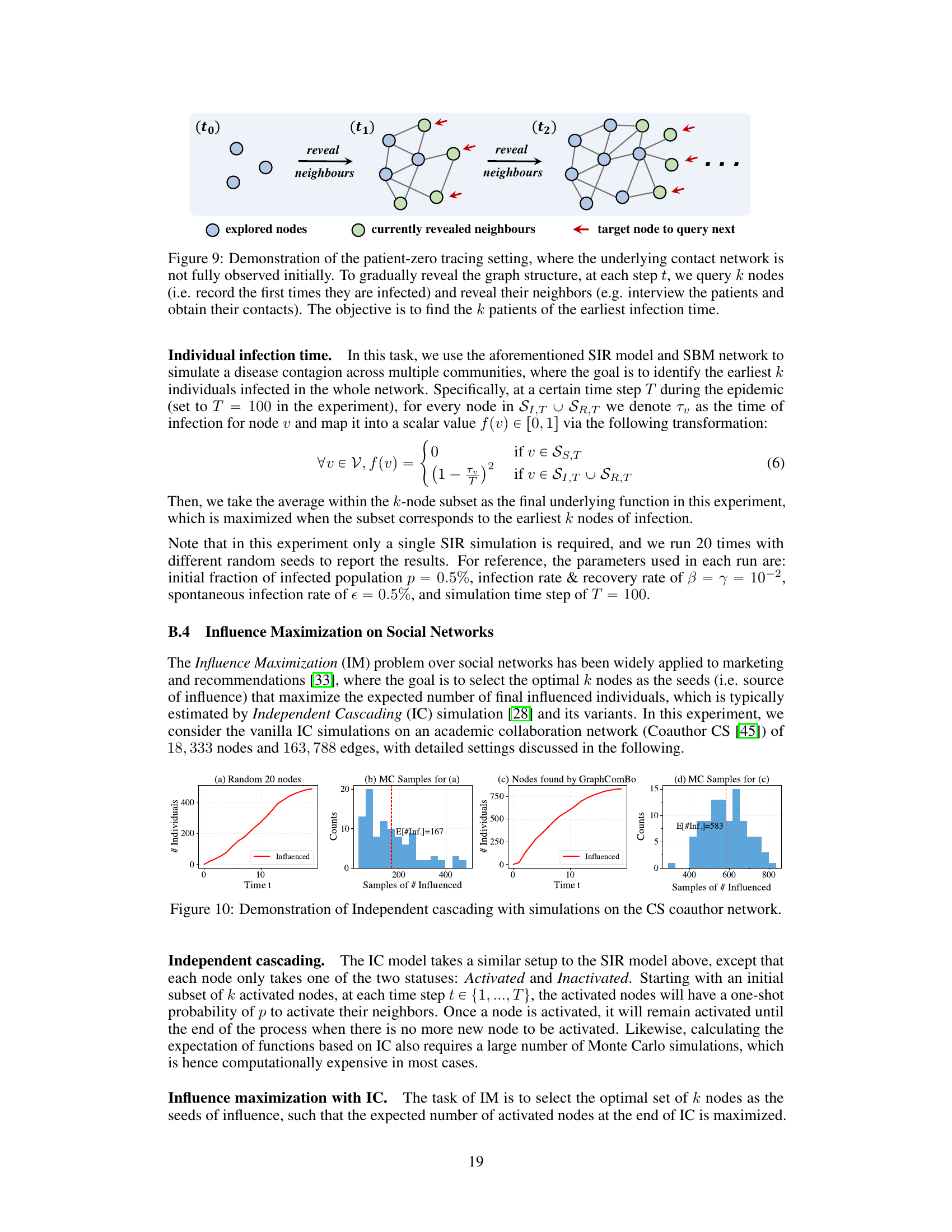
This figure illustrates the process of identifying the earliest infected individuals (patient zero) in a partially observable network. It shows how the network is incrementally revealed by querying k nodes at each time step (t0, t1, t2,…). The querying process reveals the immediate neighbors of the queried nodes, expanding the known portion of the network. The goal is to identify the k nodes that were infected the earliest.

This figure demonstrates the results of the SIR (Susceptible-Infected-Recovered) simulation model applied to a real-world proximity contact network. Subfigures (a) and (b) show the results of randomly protecting 20 nodes, while (c) and (d) show the results when using the GraphComBO method to select 20 nodes for protection. The plots show the number of individuals in each status (Susceptible, Infected, Recovered) over time, as well as the distributions of the time it takes for 50% of the population to become infected (t*). GraphComBO is shown to delay the time it takes to reach 50% infection (increasing the mean from 54 to 62.7) more effectively than random selection.
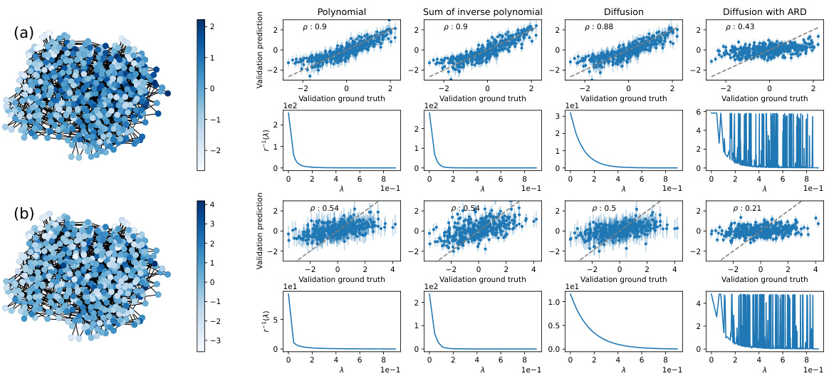
This figure shows the result of kernel validation on a Barabási-Albert network with 20 nodes and m=2. Four different kernels (Polynomial, Sum of inverse polynomial, Diffusion, Diffusion with ARD) are tested. The underlying function is created by averaging the elements of the third eigenvector over subsets of 3 nodes. The plots show the validation prediction vs. the ground truth, both without noise (a) and with added Gaussian noise (b). Spearman’s rank correlation coefficient (ρ) is given for each case.
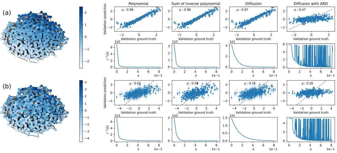
This figure displays the results of kernel validation on a Barabási-Albert (BA) network with 20 nodes and 2 edges. Two versions are shown: (a) without added noise and (b) with Gaussian noise added to the ground truth. Four different kernels (Polynomial, Sum of Inverse Polynomial, Diffusion, and Diffusion with ARD) are used and compared, with the results visualized using scatter plots and plots of the regularization functions. The underlying function is derived by averaging the elements of the third eigenvector over subsets of 3 nodes. The Spearman’s correlation coefficient (ρ) quantifies the correlation between the validation prediction and the ground truth for each kernel.

This figure visualizes the smoothness of different underlying functions used in the combinatorial space. The smoothness is evaluated by calculating the cumulative energy of Fourier coefficients, obtained via Graph Fourier Transform (GFT), of eigenvector signals from the original graph. The cumulative energy is then plotted against the eigenvalue index for different eigenvectors, demonstrating that functions corresponding to higher frequencies (larger eigenvalues) exhibit less smoothness.

This figure shows the performance of four different kernels (polynomial, polynomial_suminverse, diffusion, diffusion_ard) used in Gaussian Processes on functions with varying smoothness levels. The smoothness is controlled by using different eigenvectors from the graph Laplacian. Each boxplot shows the Spearman’s rank correlation coefficient, ρ, for each kernel on different eigenvectors (2, 4, 8, 12, 16) representing different levels of smoothness. Darker shades indicate less-smooth functions.

This figure presents a detailed behavioral analysis of the GraphComBO algorithm compared to other baselines on the task of maximizing average eigenvector centrality on Barabási-Albert (BA) networks. It shows the regret (difference between the obtained result and the optimal result), the size of the explored combo-graph, and the distance from the starting location for each algorithm. The analysis helps to understand how different algorithms explore and exploit the search space, revealing valuable insights into their exploration-exploitation strategies.
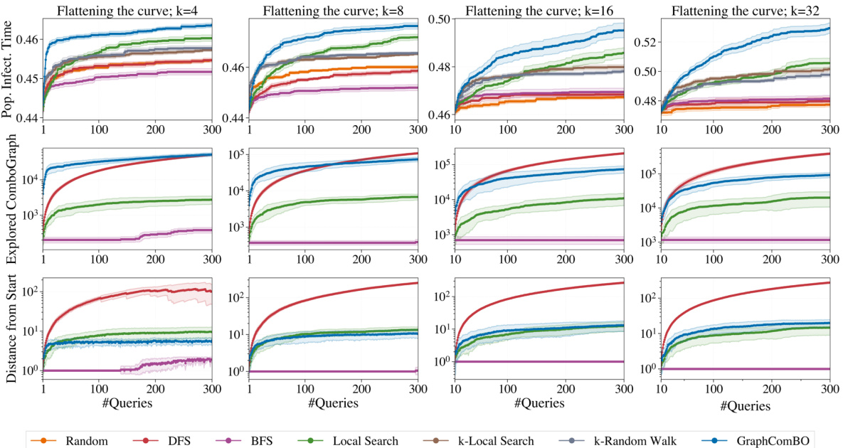
This figure presents a detailed behavior analysis of GraphComBO and other baselines on the contact network using the SIR model. It shows the performance of each method (Population Infection Time, Explored Combo-Graph Size, Distance from Start) over 300 queries for different subset sizes (k=4, 8, 16, 32). The graphs illustrate the cumulative regret, combo-graph size explored by each method, and distance traveled from the starting node over the course of 300 queries. This allows for a comparison of exploration vs. exploitation strategies.
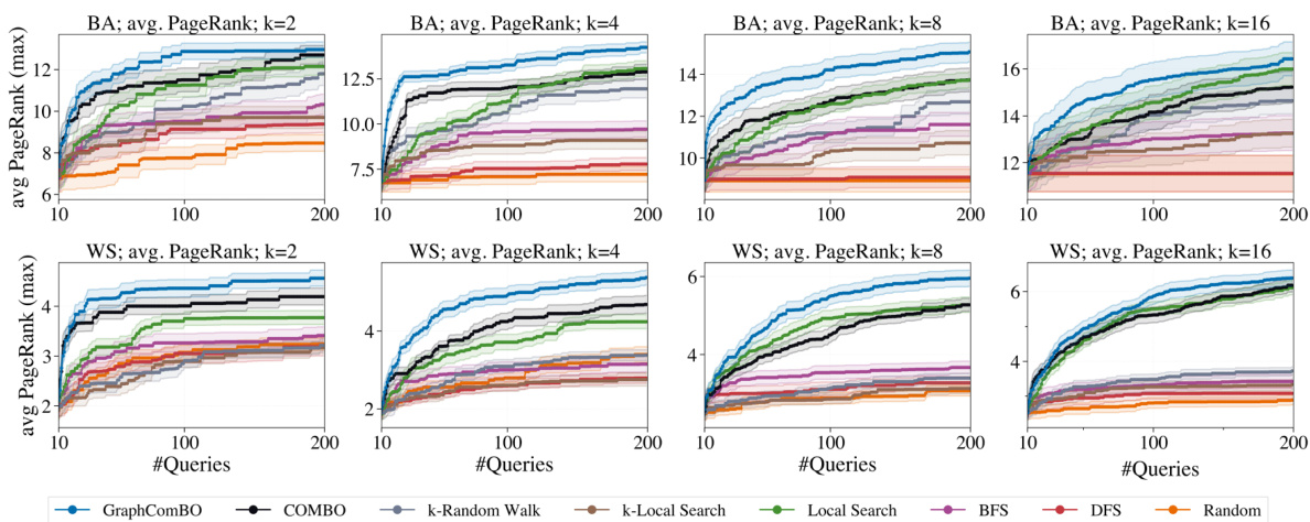
This figure compares the performance of GraphComBO with COMBO and other baselines in maximizing the average PageRank on small Barabási-Albert (BA) and Watts-Strogatz (WS) networks. The results demonstrate GraphComBO’s superior performance across different subset sizes (k). It highlights GraphComBO’s efficiency in handling the combinatorial search space compared to COMBO, especially for larger subset sizes.
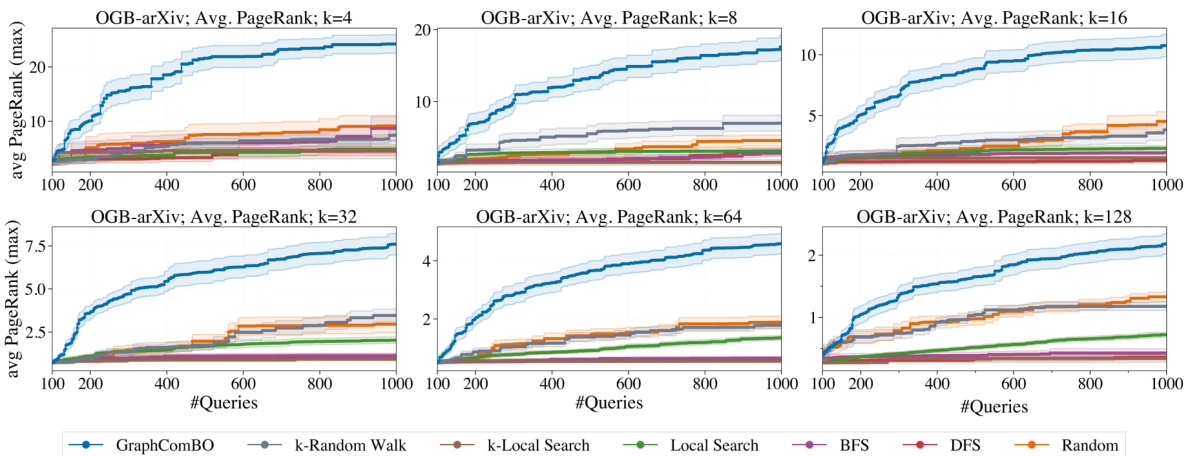
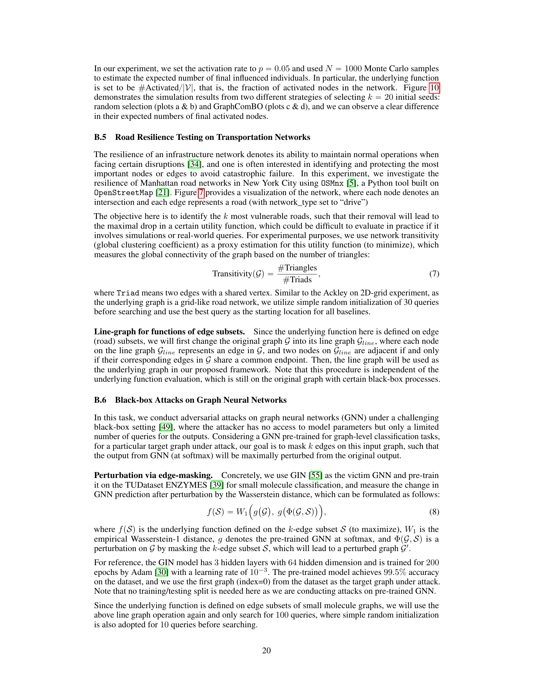
The figure shows the performance of different algorithms on a large social network (OGB-arXiv) with different subset sizes (k). It demonstrates the scalability and relative performance of GraphComBO compared to other methods like k-Random Walk, k-Local Search, Local Search, BFS, DFS, and Random search in maximizing the average PageRank score. The results highlight that GraphComBO maintains its advantage even on very large graphs.

This figure shows the density of underlying signals in the combinatorial space at different noise levels (σ = 0, 0.5, 1.0). The left panel shows the distribution for a Barabási-Albert (BA) network, and the right panel shows the distribution for a Watts-Strogatz (WS) network. The distributions illustrate how adding noise affects the smoothness and distribution of the signals, which is important for evaluating the performance of Bayesian Optimization methods in noisy environments. The original signal is shown as a blue line, and the signals with noise (σ = 0.5 and 1.0) are shown in orange and red respectively. The graphs clearly show the impact of increasing noise on the distribution of the underlying signal.
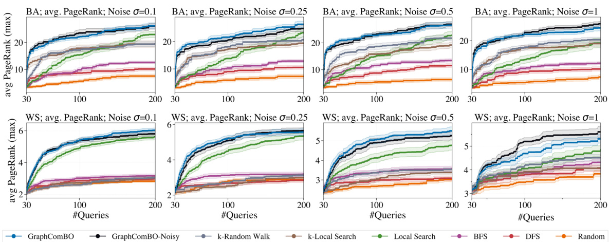
This figure shows the results of maximizing average PageRank with k=8 on Barabási-Albert (BA) and Watts-Strogatz (WS) networks under different noise levels (σ = 0.1, 0.25, 0.5, 1). It compares the performance of GraphComBO and GraphComBO-Noisy (a modification to handle noise) against several baseline methods (k-Random Walk, k-Local Search, Local Search, BFS, DFS, and Random). The plots illustrate the cumulative average PageRank achieved over multiple runs for each method and noise level. This allows for a comparison of performance under noisy conditions.
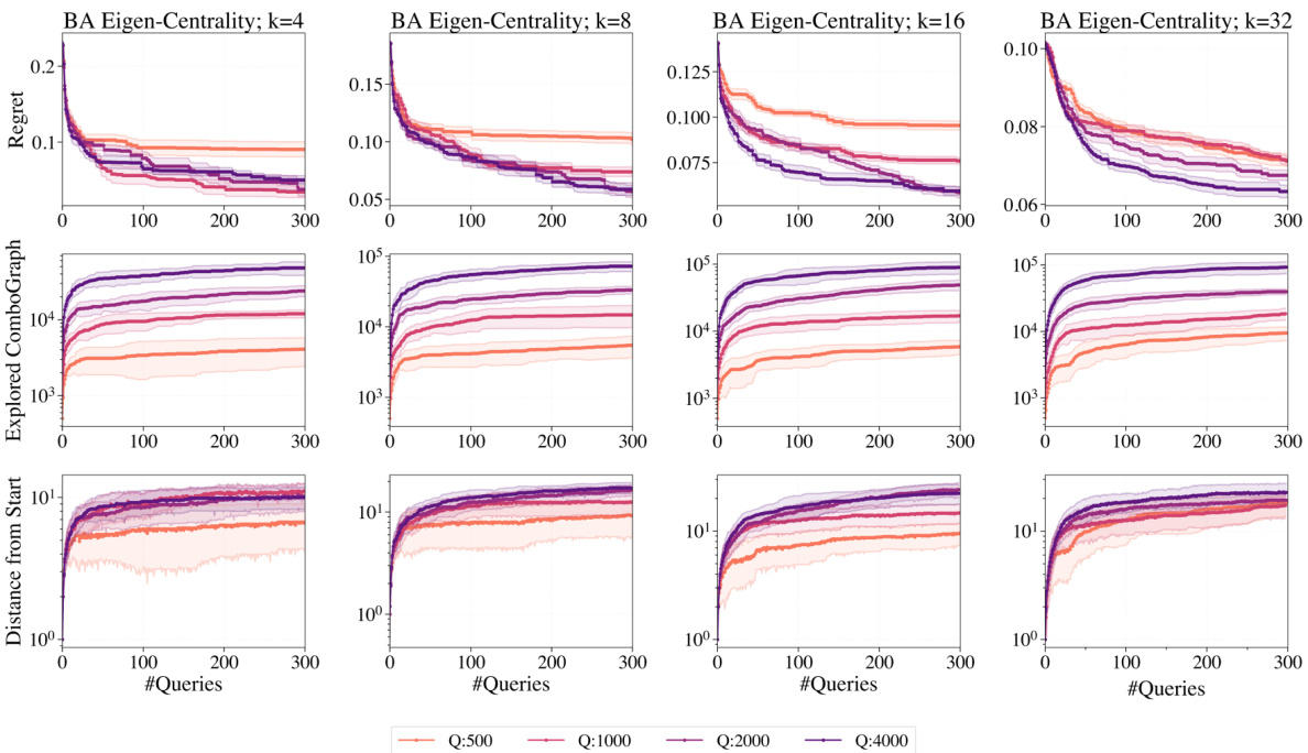
This figure shows the results of a behavior analysis of GraphComBO algorithm on Barabasi-Albert networks. It includes plots showing regret (difference between achieved value and optimal value), the size of the explored combo-graph, and the distance of the current combo-subgraph center from the starting location. Different line colors represent different values for the hyperparameter Q (the size of the local combo-subgraph sampled during the search). The purpose is to illustrate how GraphComBO explores the search space and to understand the influence of hyperparameter Q on the algorithm’s performance.
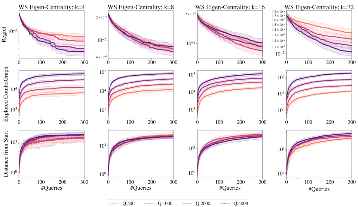
This figure shows the ablation study of the hyperparameter Q (combo-subgraph size) on Watts-Strogatz (WS) networks. The x-axis represents the number of queries, and the y-axis shows the regret (difference between the best query and the ground truth) and the explored combo-graph size. Different line colors represent different values of Q. The results show that increasing Q generally improves performance, particularly for larger values of k (subset size).
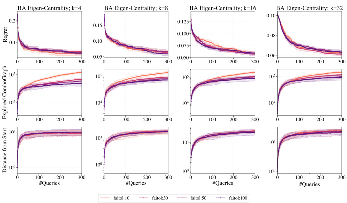
This figure presents a detailed behavioral analysis of the GraphComBO algorithm on Barabási-Albert (BA) networks for the task of maximizing average eigenvector centrality. For different subset sizes (k=4, 8, 16, 32), it shows the regret (difference between the algorithm’s best solution and the true optimum), the size of the explored combo-graph, and the distance of the current combo-subgraph center from the starting point. These metrics are tracked across various values of the failtol hyperparameter (controlling the tolerance for consecutive non-improvements). The results compare GraphComBO to other baseline methods (Random, DFS, BFS, Local Search, k-Local Search, and k-Random Walk).
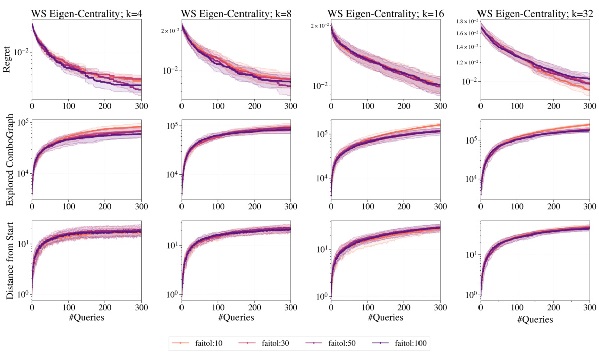
This figure provides an in-depth behavioral analysis of the GraphComBO algorithm on a real-world task of flattening the curve in an epidemic process. It shows the regret, explored combo-graph size, and the distance of the current combo-subgraph center from the starting location for different values of the hyperparameter failtol. This detailed analysis helps in understanding how the algorithm balances exploration and exploitation.
Full paper#
