Personalized Adapter for Large Meteorology Model on Devices: Towards Weather Foundation Models

llTroju97T

Shengchao Chen et el.

TL;DR
#

Accurately modeling weather patterns from complex data is crucial for timely disaster warnings and efficient resource allocation. Traditional physics-based methods and recent deep learning approaches face challenges in handling the vast amounts of data, significant heterogeneity, and limited resources on edge devices. Federated learning provides a solution but still struggles with data heterogeneity across devices.

LM-WEATHER addresses these issues. It cleverly uses pre-trained language models (PLMs) as a foundation, incorporating lightweight personalized adapters to create highly customized weather models on each device. This approach effectively fuses global knowledge with local weather patterns, ensuring high efficiency and privacy during communication. Extensive testing demonstrates LM-WEATHER’s superiority over existing methods, showcasing improved accuracy and efficiency even in limited data and out-of-distribution situations.

Key Takeaways
#

Why does it matter?
#

This paper is crucial for researchers in meteorology and AI. It bridges the gap between traditional physics-based weather modeling and modern deep learning approaches by leveraging pre-trained language models. This opens new avenues for personalized, efficient on-device weather prediction, addressing the limitations of data scarcity and resource constraints in remote locations. Its findings will likely influence future work on weather foundation models and on-device AI.

Visual Insights
#

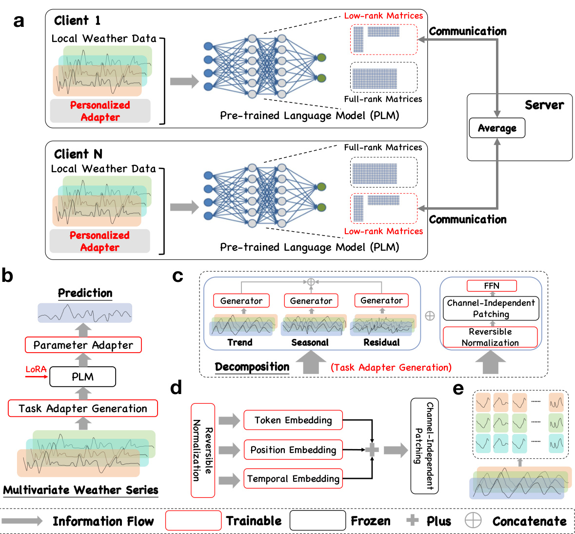
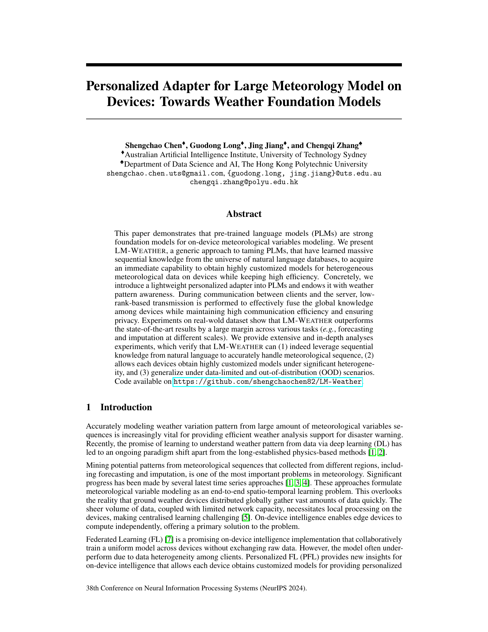
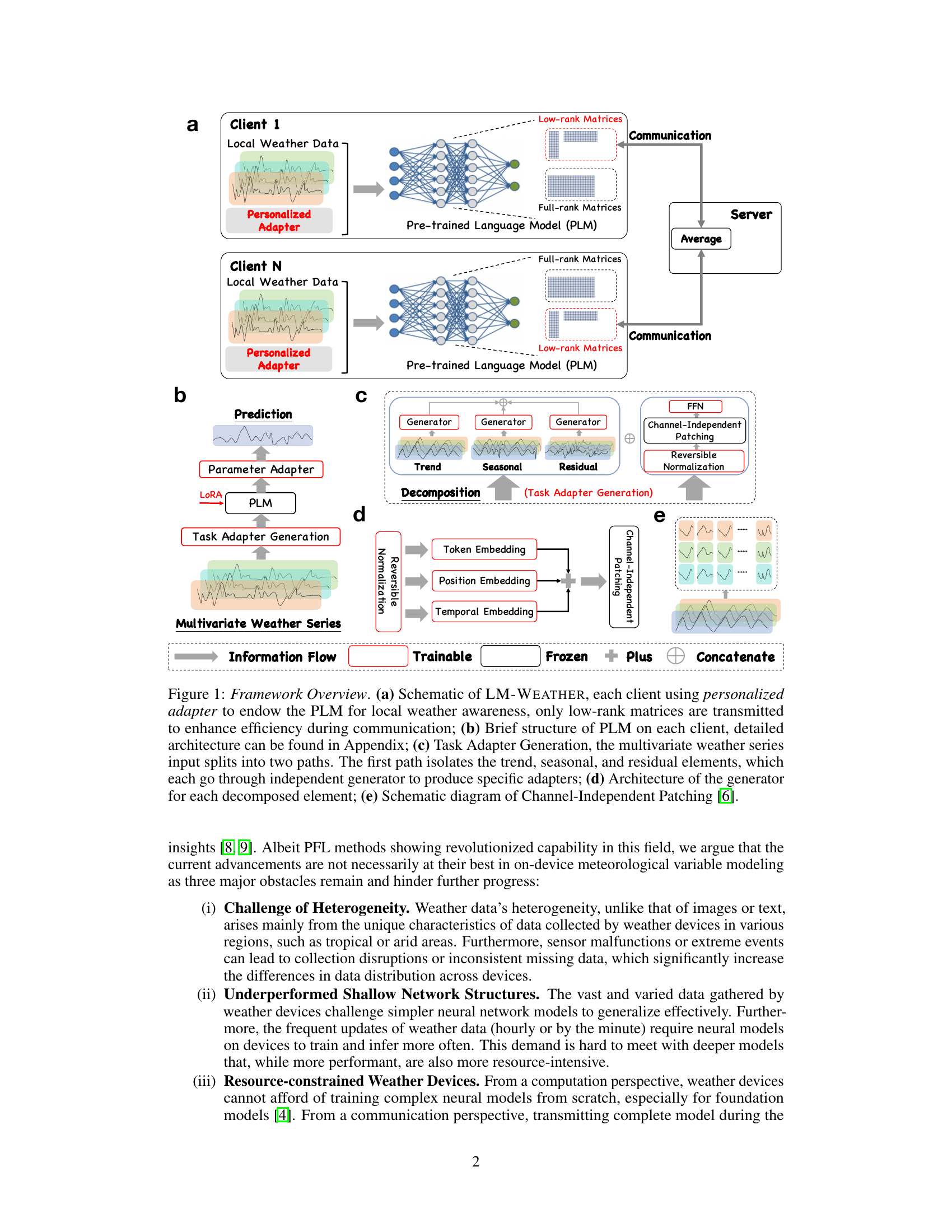
🔼 This figure provides a comprehensive overview of the LM-WEATHER framework. It illustrates the system architecture, showing how personalized adapters enhance the pre-trained language model (PLM) for each client’s specific weather data. The figure details the low-rank matrix communication strategy, the task adapter generation process (including trend, seasonal, and residual decomposition), the structure of the individual client’s PLMs, and the Channel-Independent Patching technique.
read the caption
Figure 1: Framework Overview. (a) Schematic of LM-WEATHER, each client using personalized adapter to endow the PLM for local weather awareness, only low-rank matrices are transmitted to enhance efficiency during communication; (b) Brief structure of PLM on each client, detailed architecture can be found in Appendix; (c) Task Adapter Generation, the multivariate weather series input splits into two paths. The first path isolates the trend, seasonal, and residual elements, which each go through independent generator to produce specific adapters; (d) Architecture of the generator for each decomposed element; (e) Schematic diagram of Channel-Independent Patching [6].

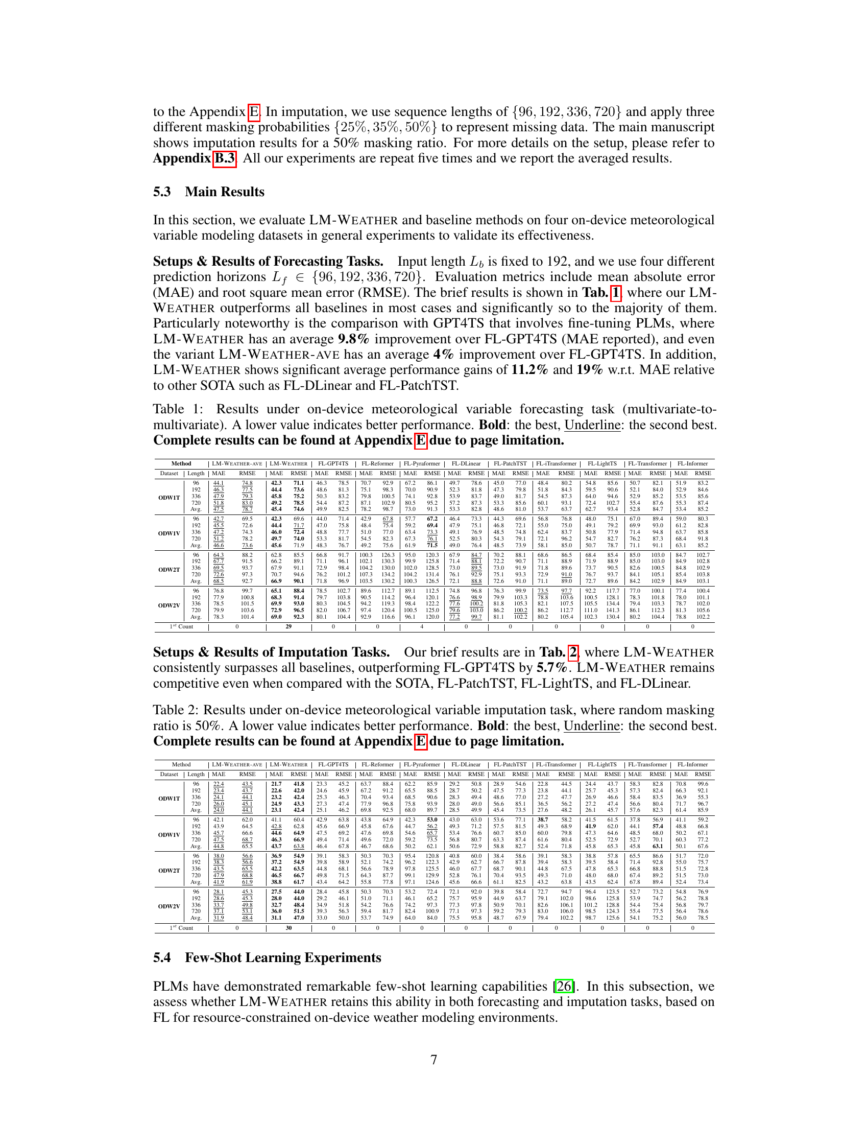
🔼 This table presents the results of a multivariate-to-multivariate forecasting experiment on on-device meteorological variable modeling. The table compares the performance of LM-WEATHER and several baselines across different prediction horizons (96, 192, 336, and 720). The evaluation metrics used are Mean Absolute Error (MAE) and Root Mean Squared Error (RMSE). The best performing model for each setting is indicated in bold, and the second best is underlined. The results demonstrate LM-WEATHER’s superior performance compared to other methods.
read the caption
Table 1: Results under on-device meteorological variable forecasting task (multivariate-to-multivariate). A lower value indicates better performance. Bold: the best, Underline: the second best.

In-depth insights
#

On-device Weather
#

On-device weather modeling presents a unique challenge due to the heterogeneity of data collected from diverse geographical locations and the resource limitations of edge devices. The paper explores using pre-trained language models (PLMs) as foundation models to create highly customized models for each device, effectively leveraging the inherent sequential understanding of PLMs to process meteorological time series. This approach addresses the heterogeneity by incorporating a lightweight personalized adapter and low-rank transmission for efficient communication. The results show improved performance on various tasks while maintaining communication efficiency and privacy, making it promising for real-world implementation. Resource constraints are a critical consideration, making the efficiency and compactness of the proposed methods a key advantage. However, further research is needed to address the data limitations for more generalized model training.

Adapter Tuning
#

Adapter tuning, in the context of large language models (LLMs) applied to weather forecasting, presents a powerful technique for achieving high accuracy while maintaining efficiency. Instead of fine-tuning the entire LLM, which is computationally expensive and resource-intensive, adapters introduce small, task-specific modules. These adapters are trained on weather data to learn the relevant patterns. This approach allows for personalized models tailored to specific weather stations or regions, taking advantage of local datasets. The key benefit is the ability to adapt existing LLMs to new tasks with minimal computational cost, overcoming the challenges of limited resources commonly associated with edge devices. Furthermore, adapter tuning can contribute to privacy enhancements, as only the smaller, adaptable modules need to be shared, reducing the transmission of sensitive data during federated learning. Low-rank matrix decomposition techniques further improve communication efficiency, allowing for effective knowledge fusion among devices with fewer data transfer requirements. However, challenges remain, such as the potential for heterogeneity in the data across different locations. A well-designed adapter tuning methodology would also carefully consider the trade-off between personalization and generalization, ensuring that highly customized models are sufficiently robust across diverse conditions.

Personalized FL
#

Personalized Federated Learning (PFL) tackles the heterogeneity challenge inherent in standard Federated Learning (FL) by creating customized models for individual clients. Unlike FL, which aims for a single global model, PFL recognizes that diverse data distributions across devices necessitate tailored approaches. This personalization enhances model performance and user experience, particularly crucial in scenarios with non-independent and identically distributed (non-IID) data. Effective PFL strategies leverage techniques like model personalization, data augmentation, and efficient communication protocols to adapt to individual client needs without sacrificing global knowledge sharing. The trade-off between personalization and global model performance requires careful consideration, as excessive personalization might compromise the global model’s generalizability. Privacy remains a critical concern, and PFL methods must ensure that sensitive user data remains protected during the training process. Overall, PFL represents a significant advancement in FL, offering greater accuracy and relevance, but demanding more sophisticated algorithms and careful consideration of the inherent complexities.

Data Efficiency
#

Data efficiency in this research paper centers around minimizing the amount of data transmitted during model training and inference, which is crucial for on-device applications. The approach uses low-rank matrices to transmit model updates, reducing communication overhead significantly. Low-rank adaptation (LoRA) is employed to update only a small number of parameters, keeping most of the model frozen. This strategy allows devices to obtain customized models while maintaining privacy. Personalized adapters are implemented to tailor the model to each device’s unique weather data. The overall strategy focuses on lightweight operations such as channel-independent patching and reversible normalization to reduce computational cost on resource-constrained devices. The use of real-world datasets, rather than simulations, adds another layer of efficiency by eliminating the need for data generation.

Future of Weather
#

The future of weather forecasting hinges on advances in computing and data science. The sheer volume of data from diverse sources, including satellites, ground stations, and simulations, requires sophisticated algorithms and powerful infrastructure to process and analyze. Artificial intelligence, particularly deep learning techniques, will play a crucial role in identifying patterns, making predictions, and improving the accuracy of forecasts, potentially leading to more precise and timely warnings of extreme weather events. Personalized forecasting, tailored to specific locations and user needs, will become more prevalent. Enhanced data assimilation techniques will further bridge the gap between model simulations and observations, improving the accuracy of weather models. Finally, the development of more comprehensive and reliable datasets covering a wide range of geographical areas and time scales will be critical for refining forecasting models and enhancing our understanding of the complex weather systems impacting our planet.

More visual insights
#

More on tables

🔼 This table presents the results of the on-device meteorological variable forecasting task. The results compare the performance of LM-WEATHER against several baselines across different prediction horizons (96, 192, 336, and 720) on four different datasets (ODW1T, ODW1V, ODW2T, and ODW2V). The performance is measured using Mean Absolute Error (MAE) and Root Mean Squared Error (RMSE). Bold values indicate the best performance for each setting, while underlined values indicate the second-best performance.
read the caption
Table 1: Results under on-device meteorological variable forecasting task (multivariate-to-multivariate). A lower value indicates better performance. Bold: the best, Underline: the second best.

🔼 This table presents the results of on-device meteorological variable forecasting experiments. The model, LM-WEATHER, is compared against several state-of-the-art baselines across four different datasets. The performance is measured using MAE and RMSE metrics for various prediction horizons (96, 192, 336, 720). The table highlights LM-WEATHER’s superior performance, consistently achieving the lowest MAE and RMSE values across almost all scenarios.
read the caption
Table 1: Results under on-device meteorological variable forecasting task (multivariate-to-multivariate). A lower value indicates better performance. Bold: the best, Underline: the second best.

🔼 This table presents the results of on-device meteorological variable forecasting experiments using multivariate-to-multivariate approach. The table shows the Mean Absolute Error (MAE) and Root Mean Squared Error (RMSE) for various forecasting lengths (96, 192, 336, 720) and on four different datasets (ODW1T, ODW1V, ODW2T, ODW2V). The best performing method for each scenario is highlighted in bold, while the second-best is underlined. The results demonstrate LM-WEATHER’s superior performance over several state-of-the-art baselines for on-device weather forecasting.
read the caption
Table 1: Results under on-device meteorological variable forecasting task (multivariate-to-multivariate). A lower value indicates better performance. Bold: the best, Underline: the second best.

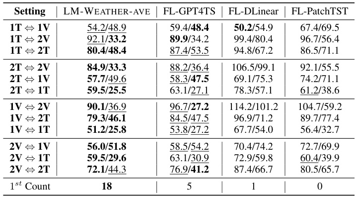
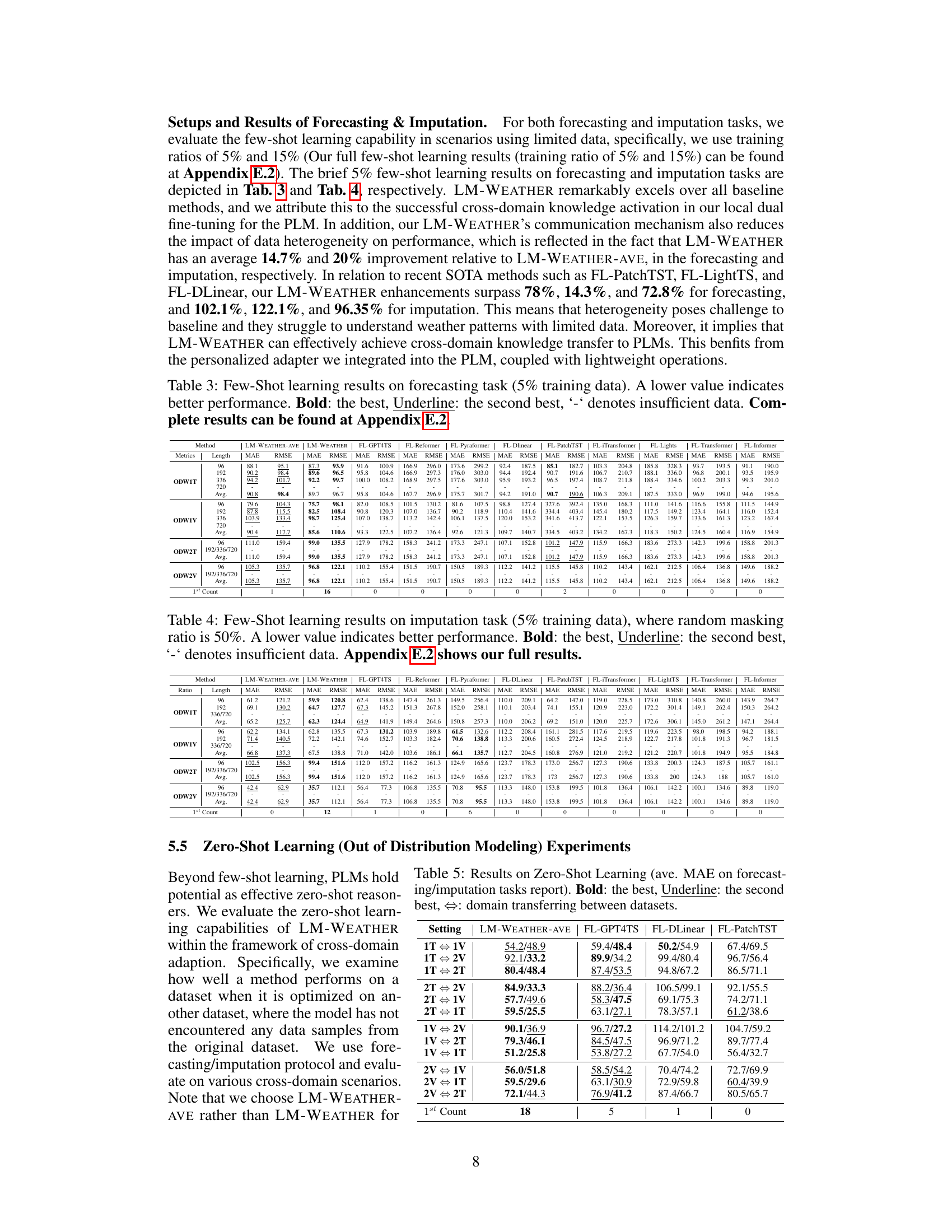
🔼 This table presents the results of a zero-shot learning experiment, where the model is evaluated on a dataset it has not been trained on. The results (average Mean Absolute Error) are shown for forecasting and imputation tasks across various scenarios. The scenarios are defined by which datasets are used for training and testing (e.g., 1T means training on ODW1T, 1V means testing on ODW1V). The table shows that LM-WEATHER-AVE outperforms other baselines across multiple scenarios in both forecasting and imputation tasks.
read the caption
Table 5: Results on Zero-Shot Learning (ave. MAE on forecasting/imputation tasks report). Bold: the best, Underline: the second best, ⇔: domain transferring between datasets.

🔼 This table presents the ablation study results for the LM-WEATHER model. It shows the impact of removing different components of the model (decomposition, trend, seasonal, residual, prompt generator) and using different methods for the personalized approach (LoRA with low-rank matrices, LoRA without low-rank matrices, full fine-tuning of attention parameters) on the performance of both forecasting and imputation tasks. The results demonstrate the importance of the weather decomposition, prompt generator, and using LoRA with low-rank matrices for achieving superior performance and efficiency.
read the caption
Table 6: Ablation results on forecasting (multivariate to multivariate) and imputation (50% masking ratio, OWD1T dataset). A lower value indicates better performance. Bold: the best, Underline: the second best, and ↑ denote performance degradation and performance improvement, respectively.

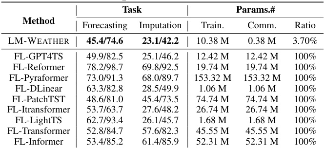
🔼 This table compares the communication efficiency and performance of LM-WEATHER against other federated learning methods designed to improve communication efficiency. It shows LM-WEATHER’s superior performance while significantly reducing the amount of data transmitted during the training process. The communication efficiency improvement is expressed as a multiplier relative to the standard approach (LM-WEATHER-Ave). MAE and RMSE metrics are also provided.
read the caption
Table 8: Comparison of LM-WEATHER and baseline that tailored to improve communication efficiency in terms of forecasting (multivariate-multivariate)/imputation (50% masking rate) performance as well as communication efficiency, with × denotes the improvement in communication efficiency relative to the standard line (LM-WEATHER-Ave), MAE/RMSE report. Bold: the best.

🔼 This table compares the performance and communication efficiency of LM-WEATHER against various federated learning baselines designed for improved communication efficiency. The metrics used are MAE and RMSE for both forecasting and imputation tasks. The communication efficiency is shown as a multiple of the standard, LM-WEATHER-Ave’s communication parameters.
read the caption
Table 8: Comparison of LM-WEATHER and baseline that tailored to improve communication efficiency in terms of forecasting (multivariate-multivariate)/imputation (50% masking rate) performance as well as communication efficiency, with × denotes the improvement in communication efficiency relative to the standard line (LM-WEATHER-Ave), MAE/RMSE report. Bold: the best.

🔼 This table presents the results of LM-WEATHER’s performance on forecasting and imputation tasks under different device participation rates. It shows how the model’s performance changes as the number of devices participating in the training increases. The results are shown for both regular training and a few-shot learning scenario where only 15% of the data is used for training. The table also highlights the increase or decrease in performance relative to the original setting (0.1 device participation rate). MAE and RMSE metrics are reported.
read the caption
Table 9: Results of LM-WEATHER under forecasting (multivariate-multivariate) and imputation (50% masking rate) at different device participation rates [0.1, 0.3, 0.5, 0.7, 0.9], ↑↓ implies an increase/decrease in performance relative to the original setting (0.1), MAE/RMSE report, where 15% represents the proportion of data on each client involved in training.

🔼 This table provides details of the ODW1T dataset, which is one of the four real-world datasets used in the paper for evaluating the proposed on-device meteorological variable modeling approach, LM-WEATHER. It lists the start and end times of the data collection period for each of the 15 weather stations in the dataset, the number of samples collected at each station, and the meteorological variables that were measured. This information is crucial for understanding the dataset’s characteristics and for reproducing the experiments.
read the caption
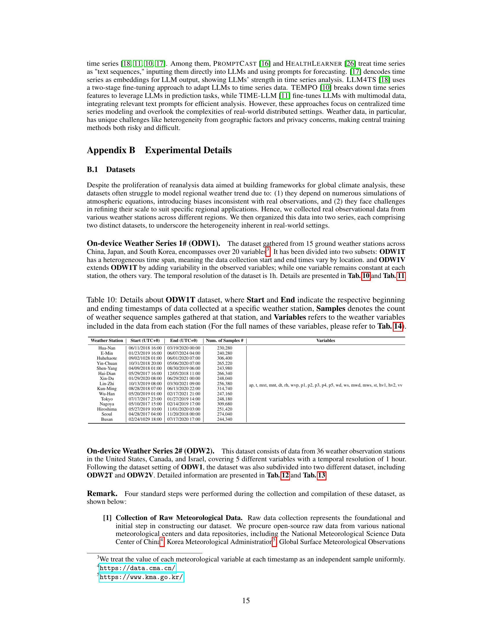
Table 10: Details about ODW1T dataset, where Start and End indicate the respective beginning and ending timestamps of data collected at a specific weather station, Samples denotes the count of weather sequence samples gathered at that station, and Variables refers to the weather variables included in the data from each station (For the full names of these variables, please refer to Tab. 14).

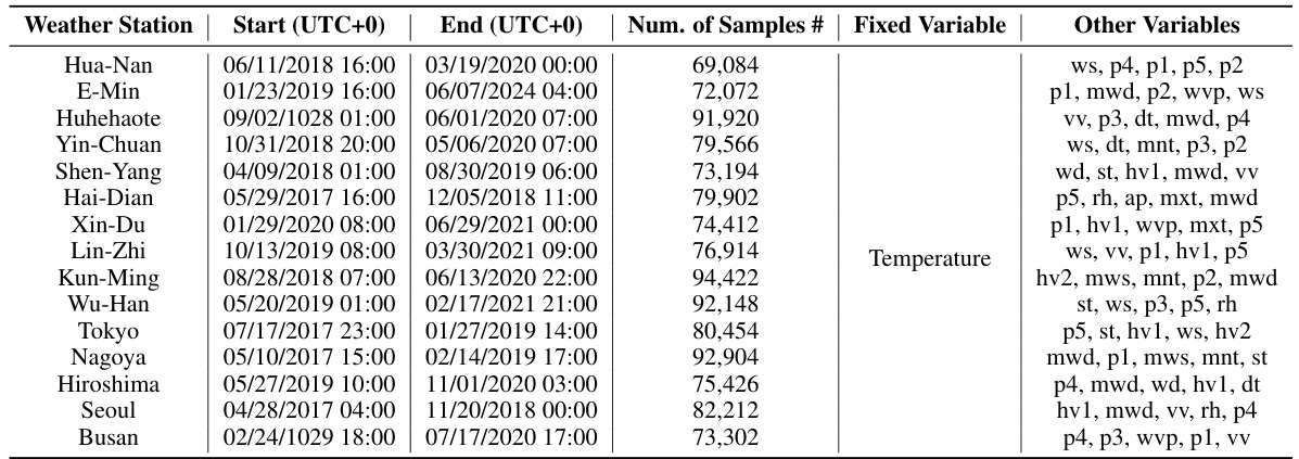
🔼 This table provides details about the ODW1T dataset, which is one of the four real-world datasets used in the paper for evaluating the performance of the proposed LM-WEATHER model. For each of the 15 weather stations included in the dataset, the table lists the start and end times of the data collection period, the number of samples collected, and the variables included. The variables are abbreviated, with the full names provided in a separate table (Table 14) in the appendix. This table highlights the heterogeneity of the data across different weather stations, in terms of both the time periods covered and the variables collected.
read the caption
Table 10: Details about ODW1T dataset, where Start and End indicate the respective beginning and ending timestamps of data collected at a specific weather station, Samples denotes the count of weather sequence samples gathered at that station, and Variables refers to the weather variables included in the data from each station (For the full names of these variables, please refer to Tab. 14).

🔼 This table shows the hyperparameters used in the experiments for LM-WEATHER. It covers different tasks (forecasting and imputation) and datasets (ODW1T, ODW1V, ODW2T, ODW2V). For each task and dataset, the table specifies the backbone model (PLM), number of layers used, training process details (patch dimension, number of heads, learning rate, loss function, batch size, local epochs), and the number of communication rounds and participation rate. The table also indicates when the few-shot learning setup (FS) is used.
read the caption
Table 17: An overview of the experimental configuration for LM-WEATHER. LR is the initial learning rate, (FS) denotes the few-shot learning setting.

🔼 This table presents the experimental configurations used in the paper for the LM-WEATHER model across different datasets (ODW1T, ODW1V, ODW2T, ODW2V). It shows the hyperparameters used for various tasks (forecasting and imputation), including the backbone PLM, number of layers, training process details (patch dimension, heads, learning rate, loss function, batch size, local epochs, communication rounds, and participation rate). The table also specifies different settings for few-shot learning scenarios.
read the caption
Table 17: An overview of the experimental configuration for LM-WEATHER. LR is the initial learning rate, (FS) denotes the few-shot learning setting.

🔼 This table presents the results of the multivariate-to-multivariate forecasting experiments conducted on four real-world datasets (ODW1T, ODW1V, ODW2T, and ODW2V). The results show the Mean Absolute Error (MAE) and Root Mean Squared Error (RMSE) for different prediction horizons (96, 192, 336, and 720) for LM-WEATHER and several baseline methods. Lower MAE and RMSE values indicate better performance. The table highlights LM-WEATHER’s superior performance across all datasets and prediction horizons, often with a significant margin over other methods. Bold values represent the best performing method, while underlined values represent the second-best performing method for each setting.
read the caption
Table 1: Results under on-device meteorological variable forecasting task (multivariate-to-multivariate). A lower value indicates better performance. Bold: the best, Underline: the second best.

🔼 This table shows the settings used for each dataset in the experiments. For forecasting, it indicates the length of the historical observation horizon used to predict future values (192 time steps in all cases). For the imputation task, which involves predicting missing values, the historical observation horizon is consistent with the prediction horizon. The table also specifies the prediction horizons used for each dataset (varying from 96 to 720 steps), as well as the random masking ratios applied for imputation (25%, 35%, or 50%).
read the caption
Table 15: Task setup for different datasets during the evaluation. Note that for the imputation task there are actually no historical observations, but rather they are performed on a single long sequence.

🔼 This table details the experimental setup for the four datasets (ODW1T, ODW1V, ODW2T, ODW2V) used in the paper. It outlines the specific tasks (forecasting and imputation) performed on each dataset, the length of the historical observation horizon used for prediction, the prediction horizons used for forecasting, and the random masking ratios used for the imputation task. The table clarifies that the imputation task doesn’t use separate historical observations but works on a single, long sequence instead.
read the caption
Table 15: Task setup for different datasets during the evaluation. Note that for the imputation task there are actually no historical observations, but rather they are performed on a single long sequence.

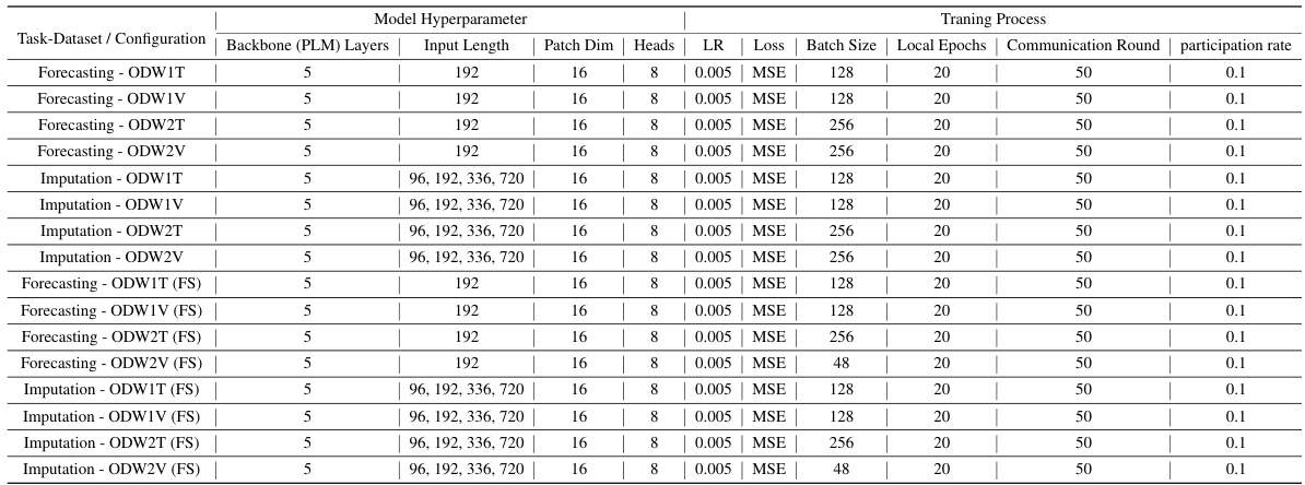
🔼 This table details the hyperparameters used in the experiments for LM-WEATHER. It shows the settings for different tasks (forecasting and imputation) and datasets (ODW1T, ODW1V, ODW2T, ODW2V). The hyperparameters include the backbone model (PLM) and the number of layers used, the input length, patch dimension, number of heads, learning rate, loss function, batch size, number of local epochs, number of communication rounds, and the participation rate. It also shows the settings for few-shot learning experiments (FS).
read the caption
Table 17: An overview of the experimental configuration for LM-WEATHER. LR is the initial learning rate, (FS) denotes the few-shot learning setting.

🔼 This table compares the performance of the proposed LM-WEATHER model against four other personalized federated learning (PFL) baselines. The comparison is done for both multivariate-multivariate forecasting and imputation tasks (with a 50% random masking rate for imputation). The ‘Avg.’ column shows the average performance across four different prediction horizons (96, 192, 336, and 720). The best performance for each metric is bolded.
read the caption
Table 18: Comparison on personalized performance between our LM-WEATHER and PFL baselines under forecasting (multivariate-multivariate) and imputation (50% masking rate), where Avg. denotes the average performance of four periods [96, 192, 336, 720], Bold means the best.

🔼 This table presents the results of the on-device meteorological variable forecasting task, specifically focusing on the multivariate-to-multivariate scenario. The results compare the performance of LM-WEATHER and other state-of-the-art methods across various settings, including different lengths of input sequences and prediction horizons. Lower values indicate better performance. The ‘Bold’ entries highlight the best-performing method in each scenario, while ‘Underlined’ entries indicate the second-best performing method.
read the caption
Table 1: Results under on-device meteorological variable forecasting task (multivariate-to-multivariate). A lower value indicates better performance. Bold: the best, Underline: the second best.

🔼 This table compares the performance of the proposed LM-WEATHER model against four other personalized federated learning (PFL) baselines on two tasks: multivariate-to-multivariate forecasting and 50% random-masking imputation. The comparison shows LM-WEATHER’s superior performance across various prediction horizons (96, 192, 336, and 720) in both tasks. The ‘Avg.’ column represents the average performance over all four horizons. The table highlights the advantages of LM-WEATHER in achieving personalized performance gains.
read the caption
Table 18: Comparison on personalized performance between our LM-WEATHER and PFL baselines under forecasting (multivariate-multivariate) and imputation (50% masking rate), where Avg. denotes the average performance of four periods [96, 192, 336, 720], Bold means the best.

🔼 This table presents the results of on-device meteorological variable forecasting experiments. It compares the performance of LM-WEATHER against several state-of-the-art baselines across four different datasets (ODW1T, ODW1V, ODW2T, ODW2V). The performance metrics used are MAE (Mean Absolute Error) and RMSE (Root Mean Squared Error) for four different prediction horizons (96, 192, 336, and 720). The best performing model for each dataset and prediction horizon is shown in bold, and the second best is underlined. The results demonstrate that LM-WEATHER outperforms the baselines across a variety of conditions.
read the caption
Table 1: Results under on-device meteorological variable forecasting task (multivariate-to-multivariate). A lower value indicates better performance. Bold: the best, Underline: the second best.

🔼 This table compares the performance of LM-WEATHER in three different settings: fully centralized training (Non-FL), federated learning with the proposed LM-WEATHER, and federated learning with only local training (LM-WEATHER-Local). The results are presented as Mean Absolute Error (MAE) and Root Mean Squared Error (RMSE) for different prediction horizons (96, 192, 336, and 720). The ‘Disparity’ row shows the percentage difference in performance compared to the fully centralized (Non-FL) training scenario.
read the caption
Table 22: Comparison of LM-WEATHER’s multivariate-multivariate performance in the FL and the Non-FL (centralised) setups, LM-WEATHER-Local is the setting in which LM-WEATHER is trained locally at each device without communication, and disparity is the difference in performance relative to Non-FL.

🔼 This table presents the results of the multivariate-to-multivariate forecasting experiments performed on four different datasets (ODW1T, ODW1V, ODW2T, ODW2V). The table shows the Mean Absolute Error (MAE) and Root Mean Squared Error (RMSE) for each dataset and for different prediction horizons (96, 192, 336, 720). The results are compared against several state-of-the-art (SOTA) baselines. The best performing model for each metric and horizon is in bold, while the second best is underlined.
read the caption
Table 1: Results under on-device meteorological variable forecasting task (multivariate-to-multivariate). A lower value indicates better performance. Bold: the best, Underline: the second best.

🔼 This table presents the results of the multivariate-to-multivariate forecasting experiments. It shows the Mean Absolute Error (MAE) and Root Mean Squared Error (RMSE) for various prediction horizons (96, 192, 336, and 720) across four different datasets (ODW1T, ODW1V, ODW2T, ODW2V). The results compare LM-WEATHER and LM-WEATHER-AVE against several state-of-the-art baselines (FL-GPT4TS, FL-Reformer, FL-Pyraformer, FL-DLinear, FL-PatchTST, FL-iTransformer, FL-LightTS, FL-Transformer, FL-Informer). The best-performing model for each metric and dataset is indicated in bold, and the second best is underlined.
read the caption
Table 1: Results under on-device meteorological variable forecasting task (multivariate-to-multivariate). A lower value indicates better performance. Bold: the best, Underline: the second best.

🔼 This table presents the results of the multivariate-to-multivariate forecasting task on four different datasets (ODW1T, ODW1V, ODW2T, ODW2V) using different prediction horizons (96, 192, 336, 720). The results are shown in terms of Mean Absolute Error (MAE) and Root Mean Squared Error (RMSE). The best performing method for each setting is bolded, and the second-best is underlined.
read the caption
Table 1: Results under on-device meteorological variable forecasting task (multivariate-to-multivariate). A lower value indicates better performance. Bold: the best, Underline: the second best.

🔼 This table presents the performance of LM-WEATHER and several baseline methods on a weather anomaly detection task using the ODW1T dataset. The performance is evaluated under two scenarios: a regular setting with the full training data and a few-shot setting with only 5% of the training data. The metrics used to evaluate performance are Precision (P), Recall (R), and F1-score (F1). The table highlights that LM-WEATHER outperforms baseline methods under both scenarios.
read the caption
Table 26: Results of LM-WEATHER and baseline for weather anomaly detection tasks on ODW1T, including regular and few-shot scenarios, where 5% means that 5% of the data is used in training, Bold and Underline denote the best and the second best.

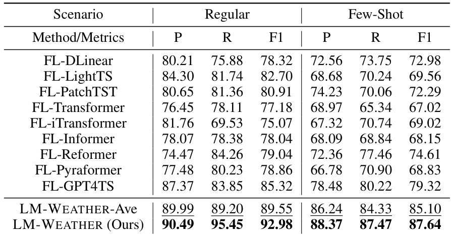
🔼 This table presents the results of a weather anomaly detection experiment. The experiment compares the performance of LM-WEATHER against several baseline methods. Two scenarios are considered: a regular scenario (with a full training dataset) and a few-shot scenario (with only 5% of the data used for training). The table reports Precision, Recall, and F1-score for each method and scenario. The goal is to evaluate the effectiveness of LM-WEATHER in detecting anomalies in weather data, particularly when only a limited amount of training data is available.
read the caption
Table 27: Results of LM-WEATHER and baseline for weather anomaly detection tasks on ODW2T, including regular and few-shot scenarios, where 5% means that 5% of the data is used in training. Bold and Underline denote the best and the second best.

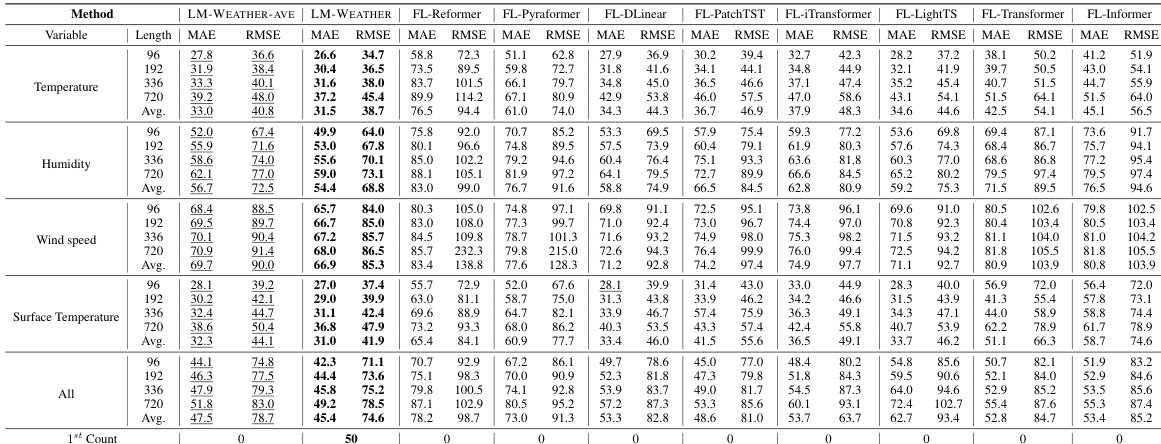
🔼 This table presents the results of on-device meteorological variable forecasting experiments where multiple variables are used for prediction. It compares the performance of LM-WEATHER and several baseline methods across various settings. Lower values of MAE and RMSE indicate better performance. The ‘Bold’ values indicate the best performance while the ‘Underlined’ values indicate second-best performance among the evaluated models.
read the caption
Table 1: Results under on-device meteorological variable forecasting task (multivariate-to-multivariate). A lower value indicates better performance. Bold: the best, Underline: the second best.

🔼 This table compares the performance and communication efficiency of LM-WEATHER against other federated learning methods optimized for communication efficiency. It shows that LM-WEATHER achieves superior performance while significantly reducing communication overhead, highlighting its efficiency in on-device weather modeling.
read the caption
Table 25: Comparison between LM-WEATHER and baseline that tailored to improve communication efficiency in terms of forecasting (multivariate-multivariate)/imputation (50% masking rate) performance as well as communication efficiency, with × denotes the improvement in communication efficiency relative to the standard line (LM-WEATHER-Ave), MAE/RMSE report. Bold: the best.

🔼 This table presents the results of the on-device meteorological variable forecasting task, specifically focusing on multivariate-to-multivariate forecasting. It compares the performance of LM-WEATHER against several state-of-the-art baseline methods across different prediction horizons and evaluation metrics (MAE and RMSE). Lower values indicate better performance. The ‘Bold’ and ‘Underline’ annotations highlight the best and second-best performing methods, respectively. This comparison helps evaluate the effectiveness of LM-WEATHER in handling complex meteorological sequences.
read the caption
Table 1: Results under on-device meteorological variable forecasting task (multivariate-to-multivariate). A lower value indicates better performance. Bold: the best, Underline: the second best.

🔼 This table compares the performance of LM-WEATHER against several baseline models for both forecasting and imputation tasks on the ODW1T dataset. It shows MAE, RMSE, model size (on device) and the communication parameters for each model. LM-WEATHER demonstrates superior performance with a smaller communication parameter size compared to the baseline models.
read the caption
Table 25: Comparison between LM-WEATHER and baseline in terms of model size on the device and performance of forecasting (multivariate-to-multivariate), and imputation (50% masking rate) on ODW1T (MAE/RMSE report), where Bold and Underline denote the best and the second best.

🔼 This table presents the results of the on-device meteorological variable forecasting task, specifically focusing on multivariate-to-multivariate forecasting. The table compares the performance of LM-WEATHER against several state-of-the-art baseline methods across different prediction horizons (96, 192, 336, 720) on four different datasets. Lower values for MAE (Mean Absolute Error) and RMSE (Root Mean Squared Error) indicate better model performance. The table highlights the best performing model in bold and the second-best model in underline for each setting. The results demonstrate the superior performance of the LM-WEATHER model compared to the baselines.
read the caption
Table 1: Results under on-device meteorological variable forecasting task (multivariate-to-multivariate). A lower value indicates better performance. Bold: the best, Underline: the second best.

🔼 This table presents the experimental setup used for LM-WEATHER. It lists various hyperparameters used for training and evaluation across different datasets and tasks, including the backbone model used (PLM), the number of layers used, the input length, patch dimension, number of heads, learning rate, loss function, batch size, local epochs, and communication rounds. The table also differentiates between regular and few-shot learning settings.
read the caption
Table 17: An overview of the experimental configuration for LM-WEATHER. LR is the initial learning rate, (FS) denotes the few-shot learning setting.

🔼 This table presents the results of the on-device meteorological variable forecasting task (multivariate-to-multivariate). The performance is evaluated using MAE and RMSE metrics. The lowest MAE and RMSE values indicate better performance. The table compares the performance of LM-WEATHER with several state-of-the-art baselines across different prediction horizons (96, 192, 336, and 720). The best-performing method for each setting is bolded, while the second-best is underlined.
read the caption
Table 1: Results under on-device meteorological variable forecasting task (multivariate-to-multivariate). A lower value indicates better performance. Bold: the best, Underline: the second best.

🔼 This table presents the results of the on-device meteorological variable forecasting task, specifically for the multivariate-to-multivariate scenario. The table compares the performance of LM-WEATHER and several other state-of-the-art methods using different prediction horizons (96, 192, 336, and 720). The metrics used for evaluation are Mean Absolute Error (MAE) and Root Mean Squared Error (RMSE). Lower values in MAE and RMSE indicate better performance. The best performing method in each scenario is bolded, and the second-best is underlined.
read the caption
Table 1: Results under on-device meteorological variable forecasting task (multivariate-to-multivariate). A lower value indicates better performance. Bold: the best, Underline: the second best.

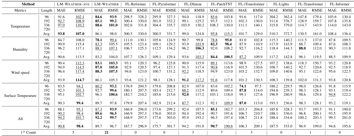
🔼 This table presents the results of the on-device meteorological variable forecasting task, specifically focusing on multivariate-to-multivariate forecasting. It compares the performance of LM-WEATHER against several state-of-the-art baselines across various settings (different lengths of input sequences and prediction horizons). Lower values in MAE and RMSE indicate better performance. The table highlights LM-WEATHER’s superior performance, consistently outperforming other models and achieving the best results across multiple settings.
read the caption
Table 1: Results under on-device meteorological variable forecasting task (multivariate-to-multivariate). A lower value indicates better performance. Bold: the best, Underline: the second best.

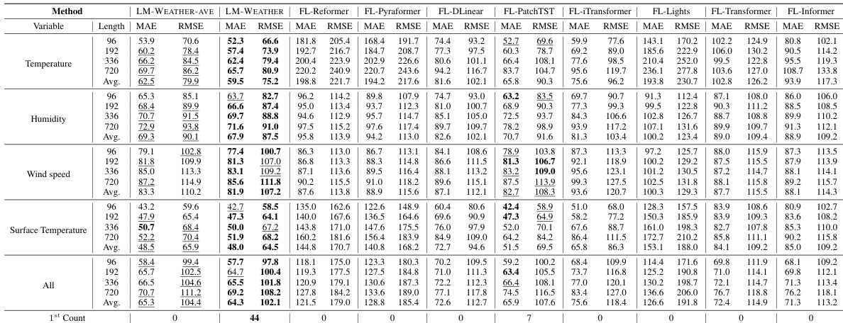
🔼 This table presents the results of the on-device meteorological variable forecasting task, specifically focusing on multivariate-to-multivariate forecasting, where multiple input variables are used to predict multiple output variables. The performance of LM-WEATHER is compared against several state-of-the-art baselines across different prediction horizons. Lower values of MAE (Mean Absolute Error) and RMSE (Root Mean Squared Error) indicate better performance. The table highlights the best-performing model (in bold) and the second-best model (underlined) for each scenario.
read the caption
Table 1: Results under on-device meteorological variable forecasting task (multivariate-to-multivariate). A lower value indicates better performance. Bold: the best, Underline: the second best.

🔼 This table provides a detailed summary of the experimental configurations used in the LM-WEATHER experiments. It outlines the hyperparameters and settings used for both forecasting and imputation tasks across different datasets (ODW1T, ODW1V, ODW2T, ODW2V). For each task and dataset, the table specifies the backbone model (PLM), the number of layers used, the training process (including patch dimension, number of heads, learning rate, loss function, batch size, local epochs, and communication rounds), and the participation rate. The table also indicates which configurations correspond to few-shot learning scenarios. This information is essential for understanding the reproducibility and comparability of the experimental results presented in the paper.
read the caption
Table 17: An overview of the experimental configuration for LM-WEATHER. LR is the initial learning rate, (FS) denotes the few-shot learning setting.

🔼 This table presents the results of the on-device meteorological variable forecasting task, specifically focusing on multivariate-to-multivariate forecasting. It compares the performance of LM-WEATHER and various baselines across four different datasets (ODW1T, ODW1V, ODW2T, ODW2V) and four different prediction horizons (96, 192, 336, 720). The metrics used for evaluation are Mean Absolute Error (MAE) and Root Mean Squared Error (RMSE). The best-performing method for each dataset and horizon is highlighted in bold, while the second-best is underlined.
read the caption
Table 1: Results under on-device meteorological variable forecasting task (multivariate-to-multivariate). A lower value indicates better performance. Bold: the best, Underline: the second best.

🔼 This table presents the results of the multivariate-to-multivariate forecasting task on four real-world datasets (ODW1T, ODW1V, ODW2T, ODW2V). The results are shown in terms of Mean Absolute Error (MAE) and Root Mean Squared Error (RMSE). Different prediction horizons (96, 192, 336, and 720) are considered. The table compares the performance of LM-WEATHER against several baseline methods including those employing federated learning (FL). Bold values indicate the best performance for each setting, while underlined values highlight the second-best performance.
read the caption
Table 1: Results under on-device meteorological variable forecasting task (multivariate-to-multivariate). A lower value indicates better performance. Bold: the best, Underline: the second best.

🔼 This table presents the results of the on-device meteorological variable forecasting task, specifically focusing on multivariate-to-multivariate forecasting. It compares the performance of LM-WEATHER against several state-of-the-art baselines across four different prediction horizons (96, 192, 336, and 720). The metrics used for evaluation are Mean Absolute Error (MAE) and Root Mean Squared Error (RMSE). Lower MAE and RMSE values indicate better performance. The table highlights the best-performing model (in bold) and the second-best performing model (underlined) for each setting.
read the caption
Table 1: Results under on-device meteorological variable forecasting task (multivariate-to-multivariate). A lower value indicates better performance. Bold: the best, Underline: the second best.

🔼 This table presents the results of imputation experiments conducted on four different real-world datasets (ODW1T, ODW1V, ODW2T, ODW2V). The evaluation metrics used are MAE (Mean Absolute Error) and RMSE (Root Mean Squared Error), and the performance is evaluated for various sequence lengths (96, 192, 336, 720) and masking ratios (25%, 35%, 50%). The table compares the performance of LM-WEATHER against several baseline methods (FL-GPT4TS, FL-Reformer, FL-Pyraformer, FL-DLinear, FL-PatchTST, FL-iTransformer, FL-LightTS, FL-Transformer, FL-Informer). Bold values indicate the best performance for each setting, and underlined values indicate the second-best performance.
read the caption
Table 2: Results under on-device meteorological variable imputation task, where random masking ratio is 50%. A lower value indicates better performance. Bold: the best, Underline: the second best.

🔼 This table presents the results of on-device meteorological variable forecasting experiments. The models were evaluated on multivariate-to-multivariate forecasting tasks using four different datasets (ODW1T, ODW1V, ODW2T, ODW2V) and prediction horizons (96, 192, 336, 720). The performance metrics are MAE and RMSE. The lowest values in each column indicate the best-performing model. Bold indicates the best performance for each row while underlined values indicate the second best.
read the caption
Table 1: Results under on-device meteorological variable forecasting task (multivariate-to-multivariate). A lower value indicates better performance. Bold: the best, Underline: the second best.

🔼 This table presents the results of the on-device meteorological variable forecasting task, specifically focusing on the multivariate-to-multivariate scenario. It compares the performance of LM-WEATHER and several baseline models (FL-GPT4TS, FL-Reformer, FL-Pyraformer, FL-DLinear, FL-PatchTST, FL-iTransformer, FL-LightTS, FL-Transformer, and FL-Informer) across different prediction horizons (96, 192, 336, 720). The MAE (Mean Absolute Error) and RMSE (Root Mean Squared Error) are used as evaluation metrics. The lowest MAE and RMSE values indicate the best-performing model for each setting. Bold values denote the best performance, and underlined values denote the second-best performance for each scenario.
read the caption
Table 1: Results under on-device meteorological variable forecasting task (multivariate-to-multivariate). A lower value indicates better performance. Bold: the best, Underline: the second best.

🔼 This table presents the results of the on-device meteorological variable forecasting task where multiple variables are used to predict multiple other variables. It compares the performance of LM-WEATHER and various baseline methods across different datasets (ODW1T, ODW1V, ODW2T, ODW2V) and prediction horizons (96, 192, 336, 720). Lower MAE (Mean Absolute Error) and RMSE (Root Mean Squared Error) values indicate better performance. The best performing model for each scenario is in bold, and the second best is underlined.
read the caption
Table 1: Results under on-device meteorological variable forecasting task (multivariate-to-multivariate). A lower value indicates better performance. Bold: the best, Underline: the second best.

🔼 This table presents the results of on-device meteorological variable forecasting experiments. The task is multivariate-to-multivariate forecasting, meaning multiple meteorological variables are used to predict multiple other variables. The table compares the performance of LM-WEATHER and several baseline methods across four different prediction horizons (96, 192, 336, 720) and the average performance. Lower MAE and RMSE values indicate better performance. Bold values indicate the best performing method for each scenario, while underlined values show the second-best.
read the caption
Table 1: Results under on-device meteorological variable forecasting task (multivariate-to-multivariate). A lower value indicates better performance. Bold: the best, Underline: the second best.

🔼 This table compares the performance and communication efficiency of LM-WEATHER against various federated learning baselines designed to improve communication efficiency. The metrics used are Mean Absolute Error (MAE) and Root Mean Squared Error (RMSE) for both forecasting and imputation tasks. The table highlights the significant improvement in communication efficiency achieved by LM-WEATHER while maintaining superior performance compared to the baselines.
read the caption
Table 25: Comparison between LM-WEATHER and baseline that tailored to improve communication efficiency in terms of forecasting (multivariate-multivariate)/imputation (50% masking rate) performance as well as communication efficiency, with × denotes the improvement in communication efficiency relative to the standard line (LM-WEATHER-Ave), MAE/RMSE report. Bold: the best.

🔼 This table presents the results of a weather anomaly detection experiment conducted on the ODW1T dataset. The experiment compares the performance of the LM-WEATHER model against several baseline methods. The results are shown for both regular training scenarios (using the full dataset) and few-shot learning scenarios (using only 5% of the dataset). Performance is evaluated using Precision, Recall, and F1-Score metrics.
read the caption
Table 26: Results of LM-WEATHER and baselines for weather anomaly detection tasks on ODW1T, including regular and few-shot scenarios, where 5% means that 5% of the data is used in training, Bold and Underline denote the best and the second best.

🔼 This table presents the results of on-device meteorological variable forecasting experiments. The experiments used a multivariate-to-multivariate setup, meaning multiple variables were used to predict multiple other variables. The results are shown for four different datasets (ODW1T, ODW1V, ODW2T, ODW2V), with results presented for multiple prediction horizons (96, 192, 336, 720). The table compares the performance of LM-WEATHER and several baseline methods, using MAE and RMSE as evaluation metrics. The best performing method for each set of parameters is bolded and the second-best is underlined.
read the caption
Table 1: Results under on-device meteorological variable forecasting task (multivariate-to-multivariate). A lower value indicates better performance. Bold: the best, Underline: the second best.

🔼 This table presents the results of a multivariate-to-multivariate forecasting experiment on on-device meteorological variable modeling. It compares the performance of LM-WEATHER and several baseline models across four different datasets (ODW1T, ODW1V, ODW2T, ODW2V) and four prediction horizons (96, 192, 336, 720). The metrics used to evaluate the models are Mean Absolute Error (MAE) and Root Mean Squared Error (RMSE). The table highlights the best and second-best performing models for each task and dataset. Lower values in MAE and RMSE indicate better performance.
read the caption
Table 1: Results under on-device meteorological variable forecasting task (multivariate-to-multivariate). A lower value indicates better performance. Bold: the best, Underline: the second best.

🔼 This table compares the communication efficiency and performance of LM-WEATHER against other federated learning baselines designed to improve communication efficiency. It shows that LM-WEATHER significantly outperforms these baselines in terms of both metrics (MAE and RMSE for forecasting and imputation) while using considerably fewer parameters for communication.
read the caption
Table 8: Comparison of LM-WEATHER and baseline that tailored to improve communication efficiency in terms of forecasting (multivariate-multivariate)/imputation (50% masking rate) performance as well as communication efficiency, with × denotes the improvement in communication efficiency relative to the standard line (LM-WEATHER-Ave), MAE/RMSE report. Bold: the best.

🔼 This table presents the hyperparameters used in the experiments of LM-WEATHER. It shows the configuration for different tasks (forecasting and imputation) and datasets (ODW1T, ODW1V, ODW2T, ODW2V). The table specifies the backbone PLM used (with the number of layers), the training process (including patch dimensions, number of attention heads, learning rate, loss function, batch size, local epochs, communication rounds, and participation rate). It also includes settings for few-shot learning experiments.
read the caption
Table 17: An overview of the experimental configuration for LM-WEATHER. LR is the initial learning rate, (FS) denotes the few-shot learning setting.

🔼 This table details the experimental setup for LM-WEATHER across various tasks and datasets. It shows the hyperparameters used for each experiment including the specific backbone PLM (pre-trained language model) and its number of layers, the training process (including patch dimensions, number of heads, learning rate, loss function, batch size, local epochs, communication rounds and participation rates). It also shows the settings for both regular training and few-shot learning.
read the caption
Table 17: An overview of the experimental configuration for LM-WEATHER. LR is the initial learning rate, (FS) denotes the few-shot learning setting.

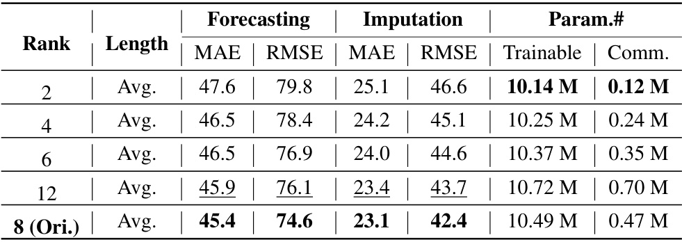
🔼 This table presents the results of a parameter impact study conducted to determine the optimal rank for the low-rank adaptation (LoRA) technique used in the LM-WEATHER model. The study varied the rank of the LoRA matrices (2, 4, 6, 12) and measured the impact on forecasting and imputation performance using MAE and RMSE metrics across different sequence lengths (96, 192, 336, 720). The table also shows the number of trainable parameters and the number of communication parameters for each rank.
read the caption
Table 54: Results on parameter impact study, where Length refers to the length of weather sequences (that is, predicted horizons in forecasting and input sequence length in imputation). Avg. represents the average value of predicted horizons, encompassing {96, 192, 336, 720}.

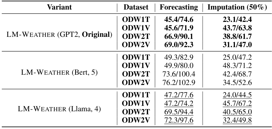
🔼 This table presents the average forecasting and imputation performance of LM-WEATHER using three different pre-trained language models (PLMs) as backbones: GPT2, Bert, and Llama. The results are averaged across all prediction horizons (96, 192, 336, and 720 time steps) for the forecasting task and across all datasets (ODW1T, ODW1V, ODW2T, and ODW2V). For the imputation task, a fixed 50% masking ratio was used. The table highlights how the choice of PLM impacts the model’s performance.
read the caption
Table 55: Performance statistics for the proposed LM-WEATHER with various PLM backbones are presented, recording only the average performance across all lengths for different datasets (namely, 96/192/336/720 prediction horizons). For the imputation task, results are documented solely for a random masking probability of 50%. Bold: the best, Underline: the second best.

TL;DR#

Key Takeaways#

Why does it matter?#

Visual Insights#

In-depth insights#

On-device Weather#

Adapter Tuning#

Personalized FL#

Data Efficiency#

Future of Weather#

More visual insights#

Full paper#