A Framework for Bilevel Optimization on Riemannian Manifolds

↗ OpenReview ↗ NeurIPS Homepage ↗ Chat

TL;DR

#

Key Takeaways

#

Why does it matter?

#

This paper is crucial for researchers working with optimization problems on manifolds, a rapidly growing area in machine learning and related fields. It offers a novel and efficient framework that addresses limitations of existing approaches, providing theoretical guarantees and practical applications. This work opens avenues for research in stochastic optimization, Riemannian geometry, and diverse machine learning tasks involving structured data.

Visual Insights

#

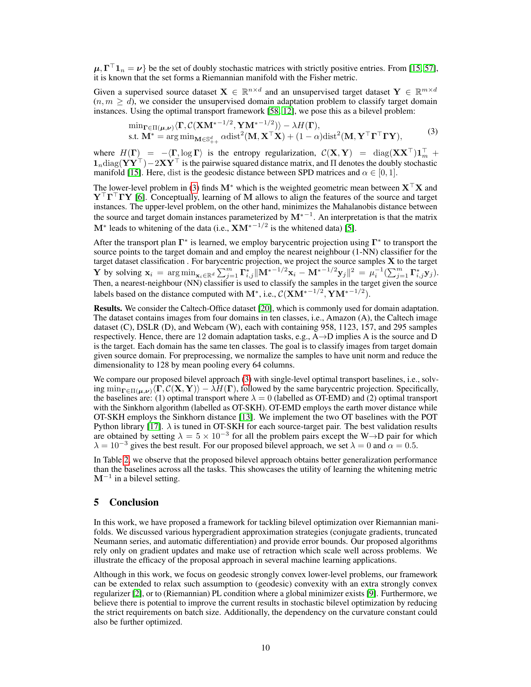
This figure presents the results of a synthetic experiment comparing different hypergradient estimation strategies for Riemannian bilevel optimization. Subfigure (a) shows the upper-level objective function over epochs for the different methods (Hessian inverse (HINV), conjugate gradient (CG), truncated Neumann series (NS), and automatic differentiation (AD)). Subfigure (b) displays the same objective but plots it against time. Subfigure (c) shows the hypergradient estimation error for these methods across epochs. Finally, subfigure (d) investigates the robustness of the NS method to changes in hyperparameters γ (damping factor) and T (number of iterations).

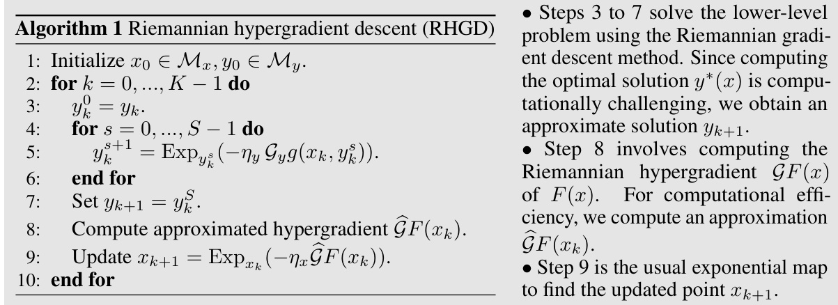
This table compares the computational complexities of different first-order and second-order methods for achieving ( \epsilon )-stationarity in bilevel optimization problems. It shows the complexities in terms of gradient computations for the upper-level function (Gf), the lower-level function (Gg), the second-order cross derivative (JVg), and the Hessian-vector product (HVg). The table distinguishes between deterministic and stochastic algorithms.

In-depth insights

#

Manifold Bilevel Opt

#

Manifold Bilevel Optimization represents a significant advancement in optimization techniques by extending bilevel programming to Riemannian manifolds. This approach is particularly valuable because it allows for the optimization of problems where both the upper and lower level variables reside in curved spaces, such as those found in machine learning applications involving SPD matrices or Stiefel manifolds. The key advantage is leveraging the inherent geometric structure of these manifolds to improve efficiency and convergence properties. The framework often involves deriving intrinsic Riemannian hypergradients, which requires careful consideration of differential geometry concepts. Various estimation strategies are typically explored, each with associated computational complexity and error bounds, such as using Hessian inverses, conjugate gradient methods, or automatic differentiation. The resulting algorithms often demonstrate superior performance compared to their Euclidean counterparts. The methodology shows promise across numerous machine learning tasks, including hyper-representation learning, meta-learning, and domain adaptation, where data often exhibits a non-Euclidean structure. The theoretical analyses usually include convergence guarantees under suitable assumptions, such as geodesic strong convexity, ensuring the practical applicability of this research.

Hypergradient Descent

#

Hypergradient descent is a crucial algorithm for solving bilevel optimization problems, which involve optimizing an upper-level objective function that depends on the solution of a lower-level problem. The core idea is to approximate the gradient of the upper-level objective with respect to the upper-level variables, treating the lower-level solution as an implicit function of these variables. This gradient, called the hypergradient, is typically estimated using implicit differentiation or approximation methods. The challenges in hypergradient estimation include the computational cost of evaluating the hypergradient accurately and the potential for instability due to the nested optimization structure. Different estimation techniques, such as Hessian-vector products or truncated Neumann series, offer various tradeoffs between accuracy and computational efficiency. The choice of hypergradient estimation method impacts the overall convergence speed and robustness of the algorithm. Furthermore, extending hypergradient descent to Riemannian manifolds introduces additional complexities due to the curved nature of the parameter space, requiring specialized techniques for gradient computation and update rules. Therefore, careful consideration of hypergradient estimation methods is paramount for efficient and reliable bilevel optimization.

Riemannian Analysis

#

Riemannian analysis, in the context of optimization on manifolds, involves extending classical optimization techniques to spaces with a curved geometry. Key aspects include defining gradients and Hessians using the Riemannian metric, adapting gradient descent methods by incorporating parallel transport or retractions, and analyzing convergence rates under suitable curvature assumptions. The choice of retraction significantly impacts computational efficiency, and careful consideration must be given to its properties when selecting an appropriate algorithm. Theoretical analysis often focuses on establishing convergence rates and error bounds for various hypergradient estimation strategies. These analyses frequently rely on concepts like geodesic convexity, which generalizes convexity to Riemannian manifolds. Practical applications involve solving bilevel optimization problems where the variables reside in manifold spaces. This approach opens doors to addressing machine learning problems with non-Euclidean data. Overall, Riemannian analysis provides a powerful theoretical framework, offering both the tools and the insight needed to extend the reach of optimization algorithms to a wider array of complex problem domains.

Stochastic Extension

#

A stochastic extension of a bilevel optimization algorithm on Riemannian manifolds would involve adapting the deterministic algorithm to handle noisy or probabilistic data. This might entail modifying hypergradient estimation techniques to use stochastic approximations of gradients and Hessians. Convergence analysis would need to be revisited, likely focusing on expected convergence rates rather than deterministic guarantees. The algorithm’s efficiency would depend critically on the choice of mini-batch size and its effect on the bias-variance trade-off in gradient approximations. A key challenge would be managing the increased computational cost associated with stochasticity. However, the benefit would be the potential to tackle very large datasets and problems intractable with deterministic methods. The impact on the overall algorithm structure, particularly hypergradient descent, requires careful consideration. It may necessitate incorporating techniques to handle the variability introduced by stochasticity, such as variance reduction methods or specialized step size selection rules. Finally, the application of retraction instead of the exponential map could enhance computational efficiency, but its impact on the stochastic convergence needs careful analysis.

Future Works

#

Future research directions stemming from this bilevel optimization framework on Riemannian manifolds could explore several promising avenues. Extending the framework to handle more complex constraints beyond those considered in the paper, such as non-convex constraints or constraints involving multiple manifolds, would significantly broaden its applicability. Investigating alternative hypergradient estimation techniques that offer improved accuracy or computational efficiency is another key area. This could involve exploring novel techniques to approximate Hessian inverses or employing advanced optimization methods. The current work primarily focuses on deterministic settings; thus, adapting the framework for truly asynchronous or decentralized environments presents a valuable research challenge. Finally, a rigorous analysis of the impact of different retraction methods on algorithm convergence and performance is warranted. While the paper touches upon retraction, a deeper exploration of its properties within the bilevel optimization context would be highly beneficial.

More visual insights

#

More on tables

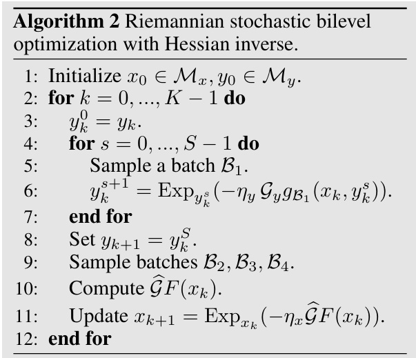
This table compares the computational complexity of different first-order and second-order methods for solving bilevel optimization problems, specifically focusing on the number of gradient and Hessian computations needed to achieve an ε-stationary point. It breaks down the complexities for deterministic and stochastic algorithms, considering the complexities of gradient calculations for both upper and lower level functions, as well as the complexities of computing second-order cross derivatives and Hessian-vector products.

This table presents the classification accuracy results achieved using three different methods: Optimal Transport with Earth Mover’s Distance (OT-EMD), Optimal Transport with Sinkhorn Divergence (OT-SKH), and the proposed Riemannian bilevel optimization approach. The results are shown for various domain adaptation tasks, represented by source and target domains (e.g., A→C means Amazon to Caltech). The proposed method demonstrates improved classification accuracy compared to the baseline optimal transport methods across all twelve adaptation tasks.

This table compares the computational complexities of different hypergradient descent methods for reaching an ε-stationary point in bilevel optimization problems. It shows the first-order and second-order complexities for both deterministic and stochastic algorithms. The complexities are broken down by the method used (Hessian Inverse, Conjugate Gradient, Neumann Series, Automatic Differentiation) and indicate gradient complexities for functions f and g, as well as complexities for computing second-order cross derivatives and Hessian-vector products.

This table compares the computational complexities of different bilevel optimization algorithms in reaching an ε-stationary point. It breaks down the complexities into first-order and second-order terms for both deterministic and stochastic methods, considering the complexities of gradient computations for both upper and lower level functions (Gf, Gg), as well as the complexities of computing second-order cross derivatives (JVg) and Hessian-vector products (HVg). The algorithms compared include several variants of Riemannian Hypergradient Descent (RHGD), along with their stochastic counterparts and a comparison against existing Euclidean algorithms.

Full paper

#