↗ OpenReview ↗ NeurIPS Homepage ↗ Chat
TL;DR#
Electroencephalography (EEG) analysis faces challenges like low signal-to-noise ratio and high inter-subject variability, hindering robust feature extraction. Existing self-supervised learning methods for EEG often struggle with these issues, leading to suboptimal performance in various applications such as brain-computer interfaces (BCIs). This necessitates more effective methods for extracting universal and reliable EEG representations.
This paper introduces EEGPT, a 10-million parameter pretrained transformer model designed to address these challenges. EEGPT employs a novel dual self-supervised learning approach combining spatio-temporal representation alignment and mask-based reconstruction. This method effectively mitigates issues related to low SNR and inter-subject variability while capturing rich semantic information. The hierarchical structure of EEGPT processes spatial and temporal information separately, enhancing flexibility and computational efficiency. Experimental results demonstrate that EEGPT achieves state-of-the-art performance on various downstream tasks, showcasing its effectiveness and scalability.
Key Takeaways#
Why does it matter?#
This paper is crucial for researchers in EEG signal processing and BCI. EEGPT offers a novel approach to extract robust and universal EEG features, addressing limitations of existing methods. Its high performance across diverse downstream tasks and potential for scalability makes it highly relevant to current research trends. The paper also opens avenues for research on improved self-supervised learning techniques and development of large-scale EEG models.
Visual Insights#
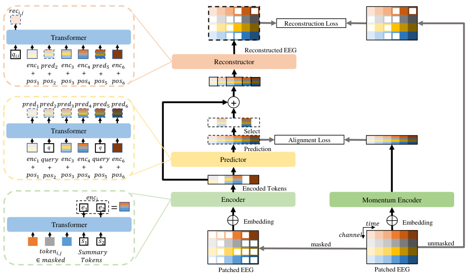
This figure shows the architecture of the EEGPT model. The input EEG signal is first divided into patches and embedded. Then, the patches are split into masked and unmasked parts. The encoder processes the masked parts to extract features, while the predictor predicts the features for the unmasked parts. The Momentum Encoder maintains a moving average of the encoder’s parameters. The reconstructor reconstructs the EEG signal from the predicted and encoded features. The alignment loss and reconstruction loss are used for training the model.
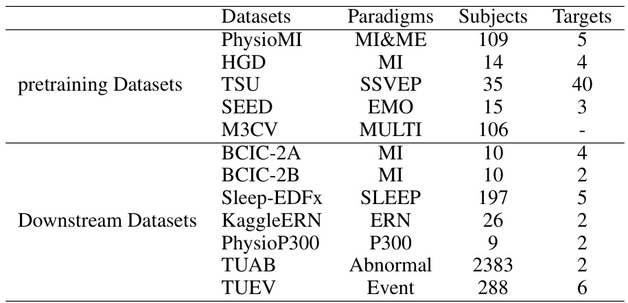
This table lists the datasets used in the EEGPT paper. It’s divided into two sections: ‘pretraining Datasets’ and ‘Downstream Datasets’. For each dataset, it provides the paradigm (type of brain activity being measured, e.g., motor imagery, emotion), the number of subjects, and the number of target classes in the data. The pretraining datasets were used to train the EEGPT model, while the downstream datasets were used to evaluate its performance on various tasks.
In-depth insights#
EEGPT Architecture#
The EEGPT architecture is a novel approach to EEG signal processing that leverages a pretrained transformer model. Its core innovation lies in a dual self-supervised learning strategy, combining mask-based reconstruction with spatio-temporal representation alignment. This dual approach allows the model to learn robust features from noisy EEG signals, mitigating the challenges of low SNR and high inter-subject variability. A hierarchical structure processes spatial and temporal information separately, leading to enhanced model flexibility and reduced computational complexity, particularly beneficial for BCI applications. The local spatio-temporal embedding method enhances compatibility with diverse EEG acquisition devices by enabling flexible adaptation to various channel configurations and sampling rates. By pretraining on a large, multi-task dataset, the model achieves universal feature extraction, demonstrating state-of-the-art performance on various downstream tasks via a linear probing approach. This architecture significantly advances EEG representation learning by addressing key limitations of existing masked autoencoder methods while offering improved scalability and robustness.
Dual Self-Supervision#
Dual self-supervised learning, as presented in this context, likely refers to a training strategy that leverages two distinct self-supervised tasks to learn robust and generalizable representations from EEG data. The method appears designed to overcome challenges inherent in EEG processing such as low signal-to-noise ratio and high inter-subject variability. One task might focus on reconstructing masked portions of the EEG signal, forcing the model to learn detailed temporal dependencies. The second task might involve some form of contrastive learning or spatio-temporal alignment, pushing the model to capture meaningful relationships across different spatial locations and time points. By combining these two approaches, the method aims to capture both fine-grained temporal details and higher-level spatial-temporal relationships within EEG signals. This dual approach is likely more powerful than using a single self-supervised task alone because it encourages the model to learn more comprehensive EEG representations, potentially resulting in improved performance on downstream tasks.
Downstream Tasks#
The ‘Downstream Tasks’ section of a research paper would detail the experiments conducted to evaluate the model’s performance on real-world applications. It would likely involve multiple tasks, each testing a different aspect of the model’s capabilities. The description should include the datasets used, the metrics employed for evaluating performance (e.g., accuracy, precision, recall, F1-score), and a thorough comparison to relevant baselines or state-of-the-art methods. A strong ‘Downstream Tasks’ section would provide convincing evidence of the model’s effectiveness and highlight its practical value. Furthermore, a discussion of the results, including any limitations or challenges encountered, would be crucial for a comprehensive understanding. The focus should be on demonstrating the generalizability of the model to various settings and tasks, showcasing its robustness and potential impact.
Scalability & Limits#
A crucial aspect of any machine learning model, especially one designed for real-world applications like EEG analysis, is its scalability. The ability to handle larger datasets, more complex models, and diverse downstream tasks is paramount. The paper’s approach, using a pretrained transformer, suggests inherent scalability due to the model’s architecture. Pretraining on a large, diverse dataset is key to achieving generalizability and robustness. However, limitations exist. Computational cost increases with model size and the complexity of downstream tasks. Linear probing mitigates some of this, but larger models could still strain resources. Furthermore, while a pretrained model offers advantages, adapting it to specific datasets and applications might demand further fine-tuning, reducing the efficiency gains of transfer learning. Data acquisition variability (quality, sampling rates, electrode placement) also poses a challenge, impacting the reliability of the learned representations. The study highlights the importance of considering scalability and resource constraints when deploying such models in real-world scenarios, particularly in resource-limited environments.
Future Research#
Future research directions for EEG-based brain-computer interfaces (BCIs) should prioritize enhancing the robustness and generalizability of EEG representations. This includes exploring advanced self-supervised learning techniques beyond the current state-of-the-art, potentially leveraging larger and more diverse datasets incorporating various recording modalities and paradigms. Addressing the challenges of low signal-to-noise ratio (SNR) and inter-subject variability remains crucial; innovative preprocessing methods and robust feature extraction techniques are needed. Furthermore, investigating the efficacy of incorporating multimodal data (e.g., fMRI, fNIRS) with EEG could significantly improve accuracy and reliability of BCIs. Finally, research should focus on developing more efficient and adaptable algorithms to better accommodate real-world BCI applications, including those with limited training data and varying conditions.
More visual insights#
More on figures
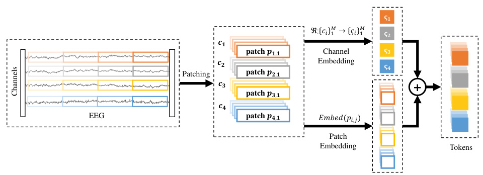
The figure illustrates the process of local spatio-temporal embedding in the EEGPT model. The EEG signal is divided into small patches across both time and channels. Each patch then undergoes linear embedding and is combined with channel-specific embedding information, resulting in a feature vector that captures both spatial (channel) and temporal information within that patch. This is a crucial step in EEGPT as it transforms the raw EEG into a format suitable for processing by the transformer model.
This figure illustrates the architecture of the EEGPT model. The input EEG signal is first divided into patches and embedded. Then, a masking process creates masked and unmasked portions. The masked part is processed by the encoder to extract features (encj), while the predictor predicts features (predj) for the whole signal, aligning them with the momentum encoder output. Finally, the reconstructor uses these features to reconstruct the original masked EEG signal, creating a dual self-supervised learning task.
The figure shows the architecture of the EEGPT model. The input EEG signal is divided into patches, and then a masking process is performed, separating patches into masked and unmasked parts. The masked patches are fed into an encoder, which extracts features, while the unmasked patches are used in a reconstruction task. A predictor network predicts the features of the masked patches, which are aligned with the output of a momentum encoder. Finally, a reconstructor uses both the predicted features and the encoder’s output to reconstruct the original EEG signal of the masked patches. This dual self-supervised learning approach is key to the model’s performance.

The figure illustrates the architecture of the EEGPT model, a transformer-based model for EEG feature extraction. The input EEG signal is first patched and split into masked and unmasked parts. The masked parts are processed by an encoder, which extracts features. A predictor then predicts features for the whole signal and these are aligned with the output of a momentum encoder. Finally, a reconstructor uses the encoder and predictor outputs to reconstruct the masked parts of the EEG signal. The whole process is a dual self-supervised learning approach with spatio-temporal representation alignment.

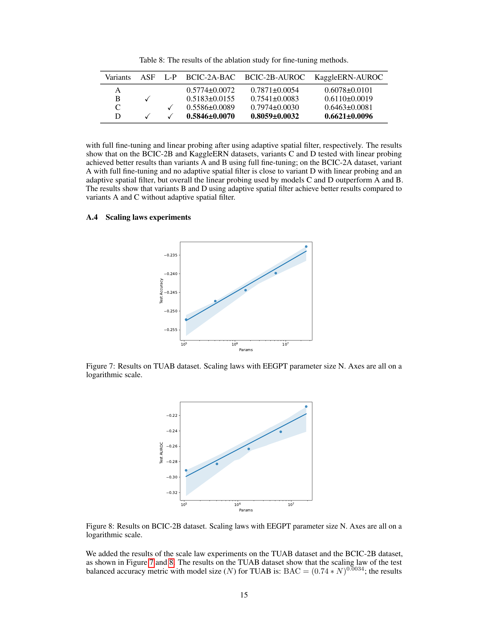
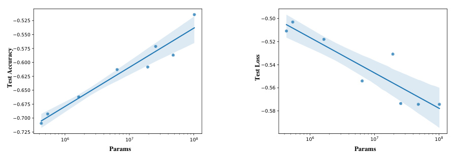
This figure shows the scaling laws observed when varying the model size (number of parameters) of the EEGPT model. The x-axis represents the number of parameters (on a logarithmic scale), and the y-axis shows two metrics: test accuracy and test loss (also on logarithmic scales). The plot demonstrates a positive correlation between model size and performance, indicating that larger models generally achieve higher accuracy and lower loss. The lines represent the trendlines fitted to the data, illustrating the relationship between model size and these performance metrics.

This figure shows the scaling laws observed when training the EEGPT model with varying parameter sizes. The x-axis represents the number of parameters in the model (log scale), while the y-axis shows both test accuracy and test loss (log scale). The plot demonstrates a positive correlation between model size and performance, indicating that larger models generally achieve higher accuracy and lower loss. The lines represent regression fits to the data, and the shaded regions represent confidence intervals. This figure supports the claim that the model scales well with increasing size, leading to improved performance.

This figure shows the scaling laws observed when varying the EEGPT model’s parameter size (N). The x-axis represents the parameter size on a logarithmic scale, while the y-axis shows both test accuracy and test loss, also on a logarithmic scale. The plot shows that as the model size increases, the test accuracy improves and test loss decreases, following clear scaling trends. These trends are quantified with the equations provided in the caption, demonstrating the relationship between model size and performance.

This figure shows the scaling laws observed during experiments on the effect of model size on EEGPT’s performance. The x-axis represents the number of parameters (model size) on a logarithmic scale, and the y-axis shows both test accuracy and test loss, also on a logarithmic scale. The lines represent the fitted curves from the experiments. This visualization demonstrates the relationship between model size and both the model’s accuracy and loss, suggesting that larger models generally lead to higher accuracy but also that larger models do not always reduce loss. The data points with error bars show that larger models yield better performance in downstream tasks.

This figure illustrates the architecture of the EEGPT model, a pretrained transformer designed for universal and reliable EEG signal representation. The model processes EEG signals by first patching and embedding them, then applying a masking strategy to create masked and unmasked parts. The masked part is fed into an encoder to extract spatio-temporal features which are then aligned with predictions from a predictor. Finally, a reconstructor utilizes both encoder and predictor outputs to reconstruct the original EEG signal, fostering dual self-supervised learning.

This figure illustrates the architecture of the EEGPT model, showing the process of patching, embedding, masking, encoding, predicting and reconstructing EEG signals using the dual self-supervised learning method. The model takes EEG signals as input, processes them through the encoder and predictor, and then uses a reconstructor to generate reconstructed signals. The spatio-temporal representation alignment and the mask-based reconstruction are also illustrated.

The figure shows the correlation between channels and motor imagery classes detected using the channel perturbation method after training on the BCIC2A dataset. Gaussian multiplicative random noise is randomly added to the signal amplitude of each channel, and the Pearson correlation between the noise intensity and changes in the corresponding class logits is calculated and presented as a heatmap. Symmetric relationships are observed for electrodes related to left and right hand movements, with bilateral electrodes corresponding to foot movements, and distinct channels corresponding to the four different classes.

This figure illustrates the architecture of the proposed EEGPT model. It shows how the input EEG signal is processed through patching, embedding, masking, and then fed into an encoder, predictor, and reconstructor. The encoder processes masked patches to extract features, the predictor predicts features aligning with the momentum encoder output, and the reconstructor uses these features to reconstruct the masked parts of the signal. The overall process is designed for efficient and effective feature extraction from EEG signals.

This confusion matrix visualizes the performance of the model on the BCIC2A dataset for classifying four motor imagery tasks: left hand, right hand, foot, and tongue. Each cell (i, j) represents the number of samples from class i that were predicted as class j. The diagonal elements show correct classifications. Off-diagonal elements indicate misclassifications. The color intensity reflects the magnitude of the values.

This figure visualizes the model’s attention distribution for the P300 task. The top section shows attention in the time period from -0.1 to 1 second, while the bottom section shows attention from 1 to 2 seconds. For each time period, it displays temporal attention, mean attention, and difference attention across various time windows. The spatial attention patterns are displayed as scalp maps for each of these attention types across the different time windows, revealing which brain regions are most relevant at different moments during the P300 task.
This figure illustrates the architecture of EEGPT, a pretrained transformer model for EEG feature extraction. It shows how the input EEG signal is processed through patching, masking, embedding, encoding (by encoder), prediction (by predictor), and reconstruction (by reconstructor), involving spatio-temporal representation alignment and mask-based reconstruction. The dual self-supervised learning method and hierarchical structure are also visually represented.
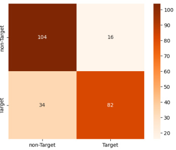
This confusion matrix visualizes the performance of the EEGPT model on the BCIC2A dataset for classifying four different motor imagery tasks: left hand, right hand, feet, and tongue. Each cell in the matrix represents the number of samples belonging to a particular class that were predicted as a specific class. The diagonal elements show the number of correctly classified samples, while the off-diagonal elements represent the misclassifications.
More on tables
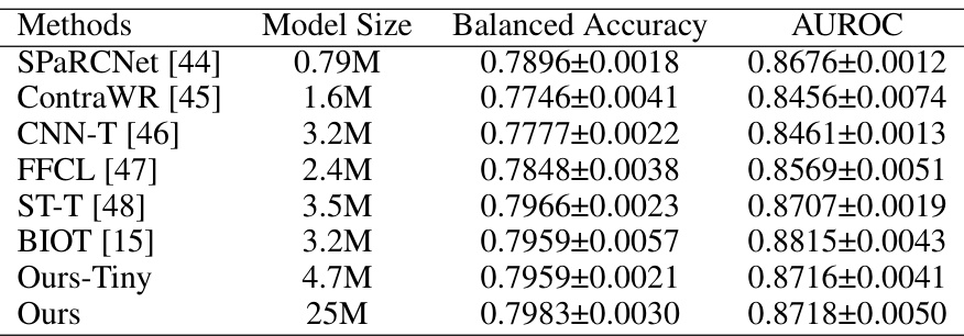
This table presents the results of various methods on the TUAB dataset for abnormal EEG detection. It compares the Balanced Accuracy (BAC) and Area Under the Receiver Operating Characteristic Curve (AUROC) achieved by several models including SPaRCNet, ContraWR, CNN-T, FFCL, ST-T, BIOT, Ours-Tiny (a smaller version of the proposed EEGPT model), and Ours (the full EEGPT model). The table shows the model size (in millions of parameters) and the performance metrics for each model. This allows for a comparison of performance across different model architectures and sizes.

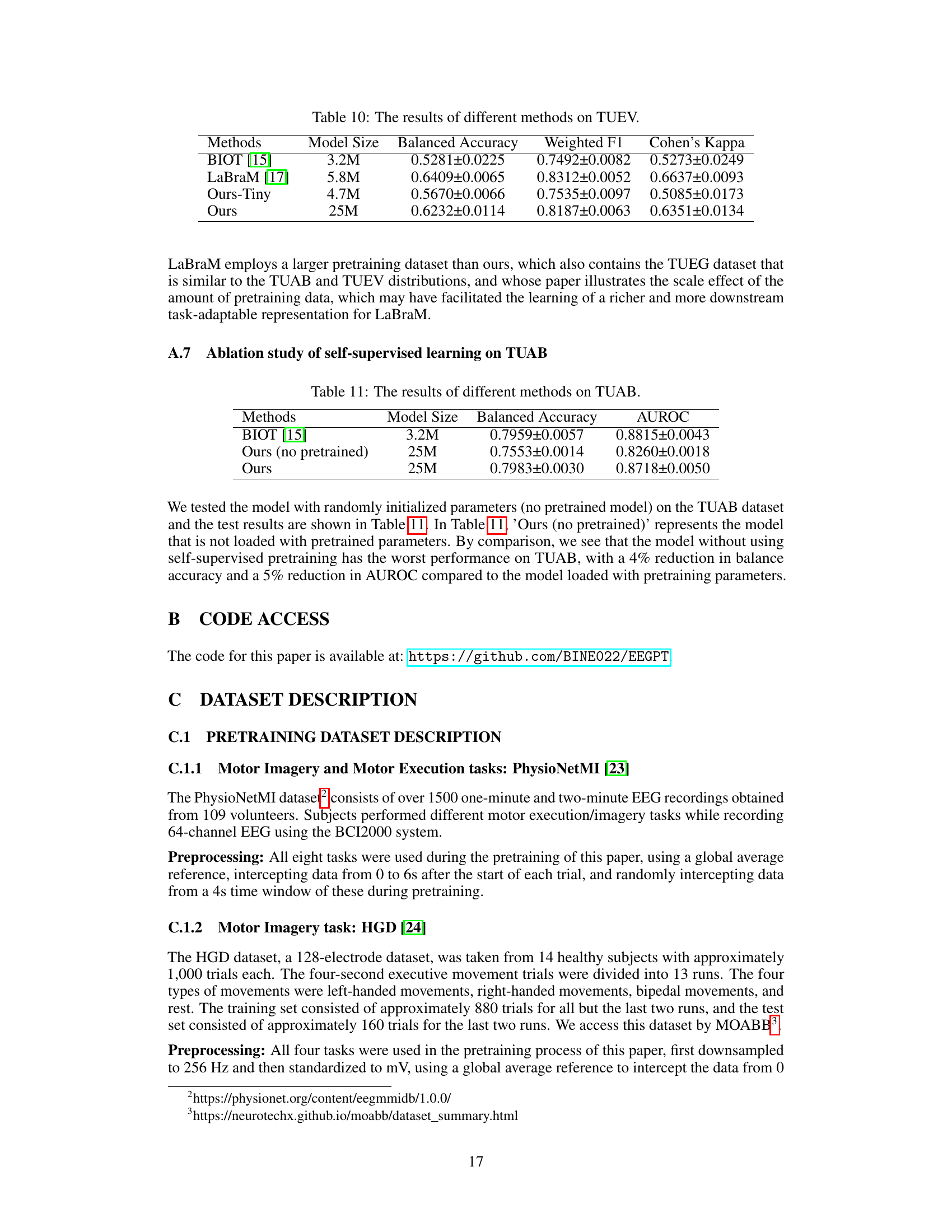
This table presents a comparison of the performance of various methods on the TUEV dataset, including the balanced accuracy, weighted F1 score, and Cohen’s kappa. The methods compared include SPaRCNet, ContraWR, CNN-T, FFCL, ST-T, BIOT, Ours-Tiny, and Ours. The model sizes are also provided for each method.

This table presents the performance of EEGPT and several other models (BENDR, BIOT, LaBraM) on various downstream tasks, including BCIC-2A, BCIC-2B, Sleep-EDFx, KaggleERN, and PhysioP300. Each row represents a different dataset, while the columns show the model used and its performance metrics: Balanced Accuracy, Cohen’s Kappa, and Weighted F1 or AUROC (area under the receiver operating characteristic curve). The results illustrate EEGPT’s ability to achieve state-of-the-art performance across multiple EEG paradigms and datasets.

This table presents the results of an ablation study on the EEGPT model’s pretraining methods. Four variants are compared: A (without spatio-temporal representation alignment loss), B (without Layer Normalization), C (without skip connection), and D (with all components). The table shows the Balanced Accuracy (BAC) on the BCIC-2A dataset, the Area Under the Receiver Operating Characteristic curve (AUROC) on the BCIC-2B dataset, and the AUROC on the KaggleERN dataset for each variant. The results demonstrate the impact of each component on the model’s performance on different downstream tasks.

This table presents the results of eight different variations of the EEGPT model trained with different hyperparameters. The variations differ in embedding dimension (de), the number of layers in the encoder, predictor, and reconstructor, and the number of summary tokens (S). The table shows the total number of parameters in each model variant, the alignment loss (LA), the reconstruction loss (LR), and the balanced accuracy achieved on the BCIC-2A dataset. The results demonstrate how different hyperparameter settings impact model performance.

This table presents the ablation study results for the pretraining methods used in the EEGPT model. It shows the balanced accuracy (BAC) on the BCIC-2A dataset, the area under the receiver operating characteristic curve (AUROC) on the BCIC-2B and KaggleERN datasets for four different model variants. Variant A excludes the spatio-temporal representation alignment loss (LA). Variant B excludes layer normalization (LN). Variant C excludes the skip connection. Variant D includes all components. The results demonstrate the importance of each component in achieving high performance.

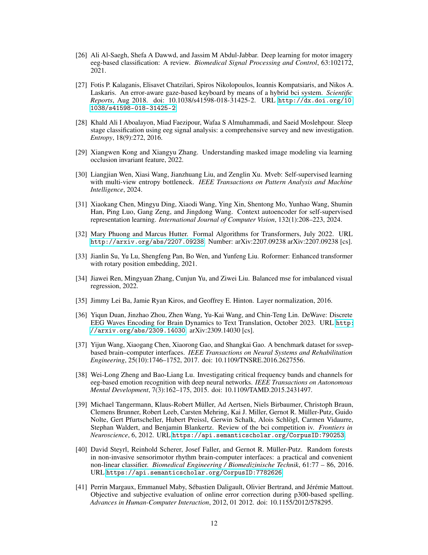
This table presents the ablation study results focusing on fine-tuning methods. It compares four model variants (A, B, C, and D) with different configurations regarding adaptive spatial filters (ASF) and linear probing (L-P). The performance is evaluated across three datasets: BCIC-2A (Balanced Accuracy), BCIC-2B (AUROC), and KaggleERN (AUROC). Variant D, which uses both adaptive spatial filters and linear probing, shows the best performance across all three datasets.

This table presents the results of different methods on the TUAB dataset for comparing the performance of EEGPT with other state-of-the-art models. It lists various models, their sizes, balanced accuracy, and AUROC scores, highlighting the performance of EEGPT in comparison.

This table presents the results of different methods on the TUEV dataset for evaluating the performance of EEGPT and other models in terms of Balanced Accuracy, Weighted F1, and Cohen’s Kappa. It compares EEGPT (both the large and a smaller ’tiny’ version) against several other state-of-the-art methods (BIOT, ST-T, FFCL, CNN-T, ContraWR, and SPaRCNet). The table allows for a direct comparison of EEGPT’s performance relative to other approaches on the same dataset. The model sizes are also listed to show the relationship between model complexity and performance.

This table presents the results of three different models on the TUAB dataset. The models compared are BIOT [15], Ours (no pretrained), and Ours. The ‘Ours (no pretrained)’ model represents the model without using pretrained parameters. The metrics used for evaluation are Balanced Accuracy and AUROC. The table shows that the pretrained ‘Ours’ model significantly outperforms the model without pretrained weights, and performs comparably to the BIOT model.

This table shows the detailed architecture of the model used for the TUAB dataset. It specifies the input size, the operators used (convolutional layers, batch normalization, GELU activation, dropout, the EEGPT encoder, flattening, and a linear layer), and hyperparameters such as kernel size, stride, groups, and padding for each layer. This architecture is designed for processing the TUAB EEG data and extracting relevant features for classification.

This table details the architecture of the model used for the TUEV dataset. It breaks down the input size, operators (layers) used, kernel size, stride, number of groups, and padding for each layer. It provides a specific configuration for processing EEG data within the context of the TUEV dataset.
Full paper#
