↗ OpenReview ↗ NeurIPS Homepage ↗ Hugging Face ↗ Chat
TL;DR#
Generative AI models, especially when used in in-context learning, often produce inaccurate or nonsensical outputs, known as hallucinations. This significantly impacts their reliability and trustworthiness, especially in high-stakes applications like finance and medicine. Current methods for evaluating and mitigating these hallucinations have limitations, making it challenging to assess and improve model performance.
This research introduces a new method to estimate the probability that a generative model will produce a hallucination, using a Bayesian framework. The core innovation lies in linking the hallucination rate to the model’s likelihood of generating a given response, requiring only the model itself, a dataset, and a query. The method is rigorously tested using large language models and synthetic data showing accuracy in predicting actual error rates, providing valuable insights into ICL and model reliability.
Key Takeaways#
Why does it matter?#
This paper is crucial for researchers working with generative AI, particularly those focused on in-context learning. It provides a novel method for quantifying the hallucination rate, a significant problem impacting the reliability of AI systems. This offers new tools for evaluating and improving the performance of these models, directly contributing to more trustworthy and robust AI applications. The Bayesian perspective employed also opens doors for further research into the underlying mechanisms of generative AI.
Visual Insights#

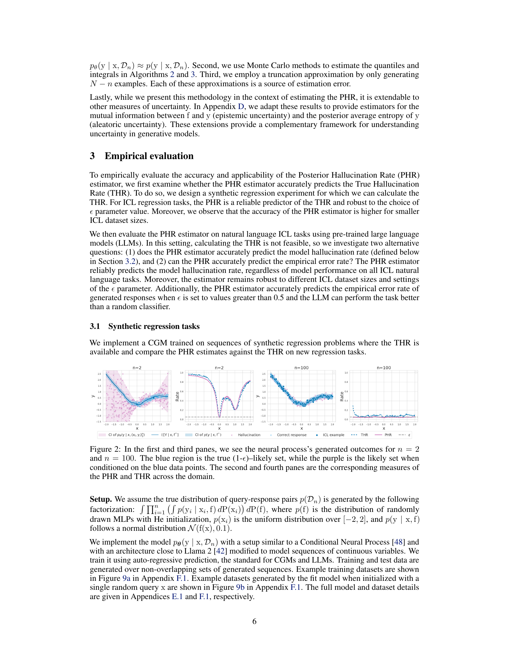
This figure shows a comparison between the true hallucination rate (THR) and the posterior hallucination rate (PHR) for different dataset sizes (n=2 and n=100). The top panels display the neural process’s generated outcomes, with the blue region representing the (1-ε)-likely set based on the true generative model and the purple region showing the (1-ε)-likely set based on the model’s posterior predictive distribution. The bottom panels illustrate the corresponding PHR and THR across the input domain. The plots demonstrate the relationship between the estimated PHR and the actual THR, particularly how the PHR’s accuracy increases as the dataset size grows, indicating the effectiveness of the proposed method for estimating hallucination rates.
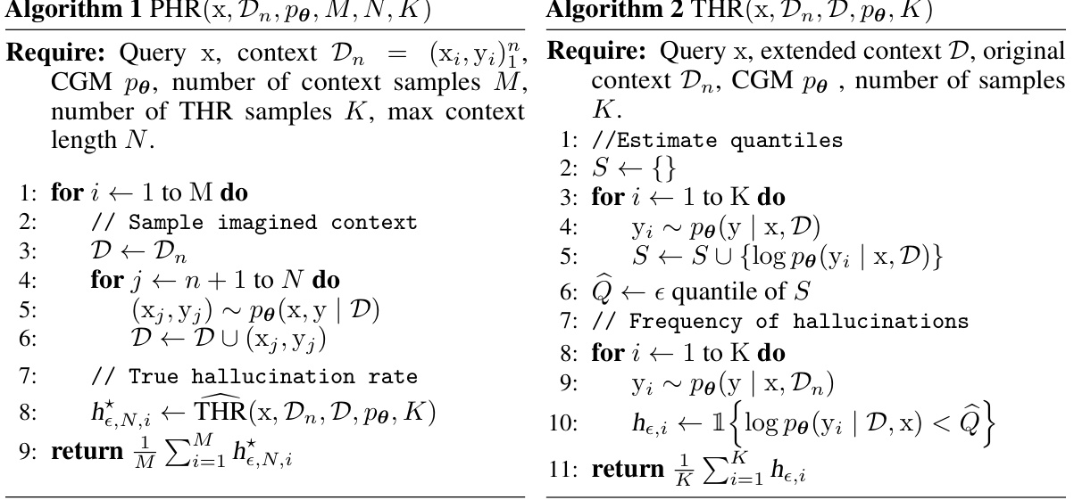
This table presents the results of an ablation study on the SST2 dataset using the Llama-2 language model. The study investigates the impact of various hyperparameters on the accuracy of the posterior hallucination rate estimator. The hyperparameters varied include the number of context samples (N-n), the number of Monte Carlo samples (M), the number of response samples (K), and the model size (number of parameters). The table shows the mean absolute error (MAE) and R-squared (R2) values for both the model hallucination rate (MHR) and the empirical error rate for each set of hyperparameter values. The results indicate that increasing the number of MC and y samples improves the R2 scores for both MHR and the empirical error rate, whereas increasing the number of generated examples or model size alone results in a performance decline.
In-depth insights#
Hallucination Rate#
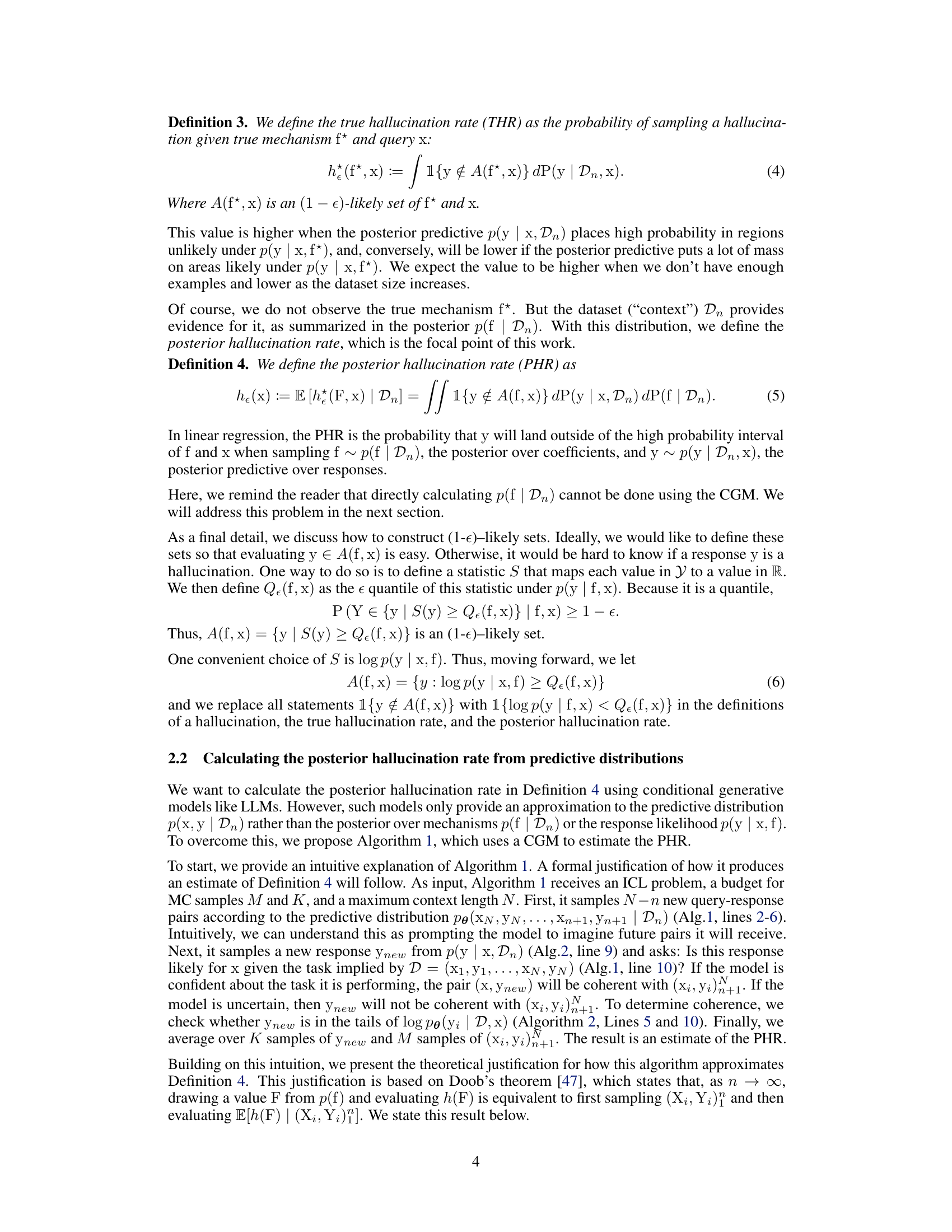
The concept of ‘Hallucination Rate’ in AI research, specifically within the context of large language models (LLMs) and in-context learning (ICL), is crucial for evaluating the reliability and trustworthiness of AI-generated content. It quantifies the frequency with which LLMs produce factually incorrect or nonsensical outputs, often termed ‘hallucinations’. The hallucination rate is not static; it varies with factors like model architecture, training data, prompt engineering, and the complexity of the task. Accurately measuring and reducing the hallucination rate is vital to enhance the reliability of LLMs for diverse applications. A key challenge lies in establishing robust and reliable methodologies for measuring this rate, since it relies on subjective judgments about what constitutes a hallucination. Further research is needed to investigate the root causes of these hallucinations, which could include biases in training data, limitations of the model’s reasoning capabilities, or even more fundamental issues in the way we frame the problem of knowledge representation and retrieval. Addressing this crucial challenge is essential for building safe, reliable, and trustworthy AI systems.
Bayesian ICL#
In the context of in-context learning (ICL), a Bayesian perspective offers a powerful framework for understanding how generative models, such as large language models (LLMs), produce predictions. The Bayesian ICL approach views the model as approximating the posterior predictive distribution of an underlying Bayesian model, implicitly defining a joint distribution over observable datasets and unobserved latent mechanisms that explain data generation. This framework enables a principled way to define hallucinations as generated responses with low likelihood given the mechanism and observed data. The key advantage of this approach lies in its ability to quantify the probability of hallucination, known as the Posterior Hallucination Rate (PHR), facilitating improved estimation of model reliability and uncertainty. By leveraging this Bayesian framework, we can move beyond simple empirical error rates and develop methods for diagnosing and mitigating model errors, thereby offering a more nuanced and insightful assessment of LLM performance. Further research can explore how different types of model uncertainty map to this Bayesian perspective, potentially leading to more effective techniques for improving the reliability of generative AI systems.
PHR Estimation#
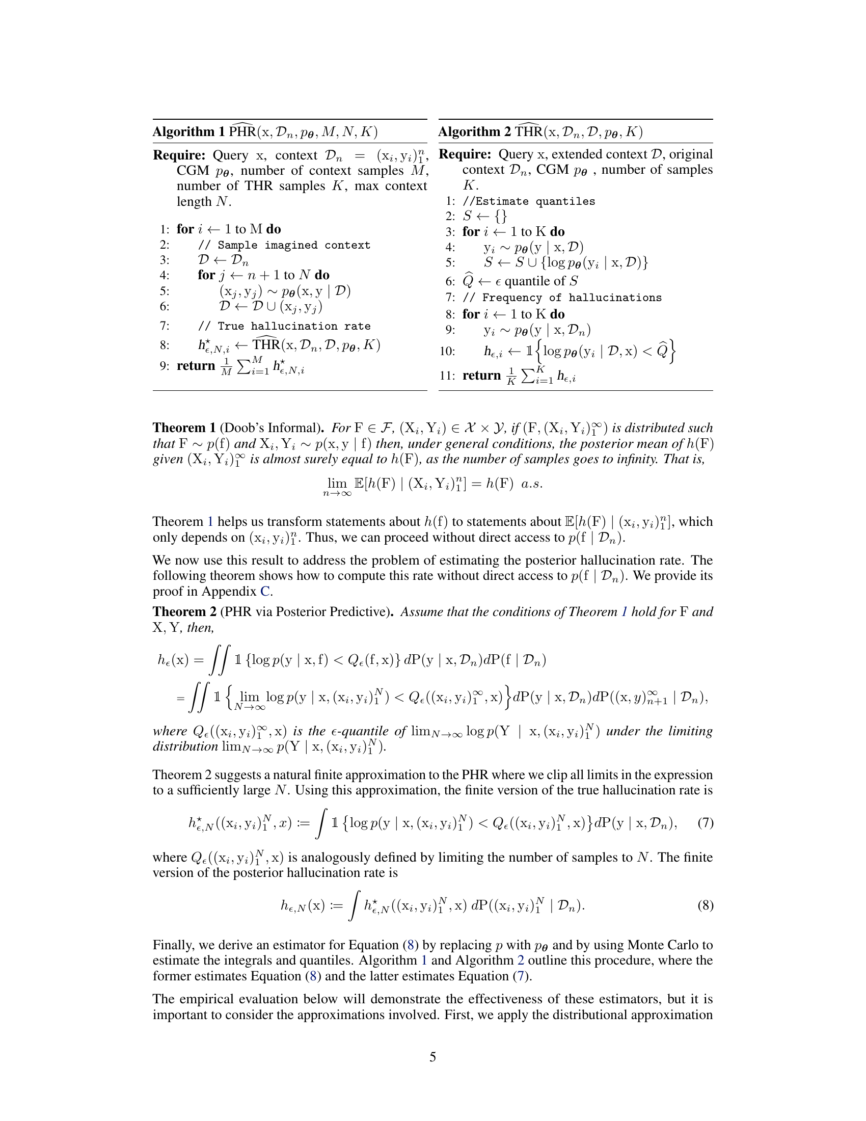
Estimating the Posterior Hallucination Rate (PHR) is a crucial aspect of the research paper, focusing on quantifying the likelihood of a generative AI model producing unreliable outputs, or ‘hallucinations’. The method proposed involves a Bayesian perspective, viewing the model’s generation as sampling from a posterior predictive distribution. The core of the PHR estimation lies in calculating the probability that a generated response falls outside a high-probability region (defined by a chosen likelihood threshold). The key innovation lies in a new method that only requires generating responses and evaluating their log-probabilities, thereby avoiding the need for auxiliary models or external information often required in similar tasks. Empirical evaluations demonstrate the effectiveness of the proposed PHR estimator, particularly in synthetic regression scenarios, showcasing its ability to accurately predict the true hallucination rate. While the method’s performance on natural language tasks is promising, limitations concerning the strict assumptions inherent in the Bayesian framework are acknowledged. Further investigation is needed to explore the robustness and generalizability of the PHR across diverse contexts and model architectures.
LLM Evaluation#
Evaluating Large Language Models (LLMs) is a complex process, demanding multifaceted approaches. Benchmark datasets play a crucial role, yet their limitations in fully capturing real-world performance must be acknowledged. Quantitative metrics, such as accuracy, BLEU score, or ROUGE, offer a convenient summary, but often fail to capture nuanced aspects of LLM output like fluency, coherence, and factual accuracy. Therefore, human evaluation remains essential, enabling assessments of aspects that are difficult to quantify. Bias and fairness are critical considerations, demanding thorough analysis of LLM outputs to detect and mitigate potential biases. Furthermore, robustness testing, evaluating LLM performance against adversarial examples or variations in input format, is critical for ensuring reliability. Finally, resource considerations, including computational costs and energy usage, are important factors when evaluating the overall impact and scalability of LLMs.
Future Work#
The paper’s conclusion points toward several promising avenues for future research. Addressing the limitations of the current PHR estimator is paramount; this includes investigating the impact of the distributional approximation made and refining the Monte Carlo methods used to reduce estimation errors and improve accuracy. Another crucial area involves exploring the interaction between aleatoric and epistemic uncertainty in the context of hallucinations. A deeper understanding of how these types of uncertainty contribute to inaccurate predictions is critical for developing more effective mitigation strategies. Furthermore, extending the methodology to account for different types of hallucinations and varying model architectures would enhance its generalizability and practicality. Finally, and perhaps most importantly, is investigating the broader social implications of accurate hallucination rate estimation. The potential for misuse of this technology underscores the importance of developing methods to enhance user awareness and promote responsible use.
More visual insights#
More on figures

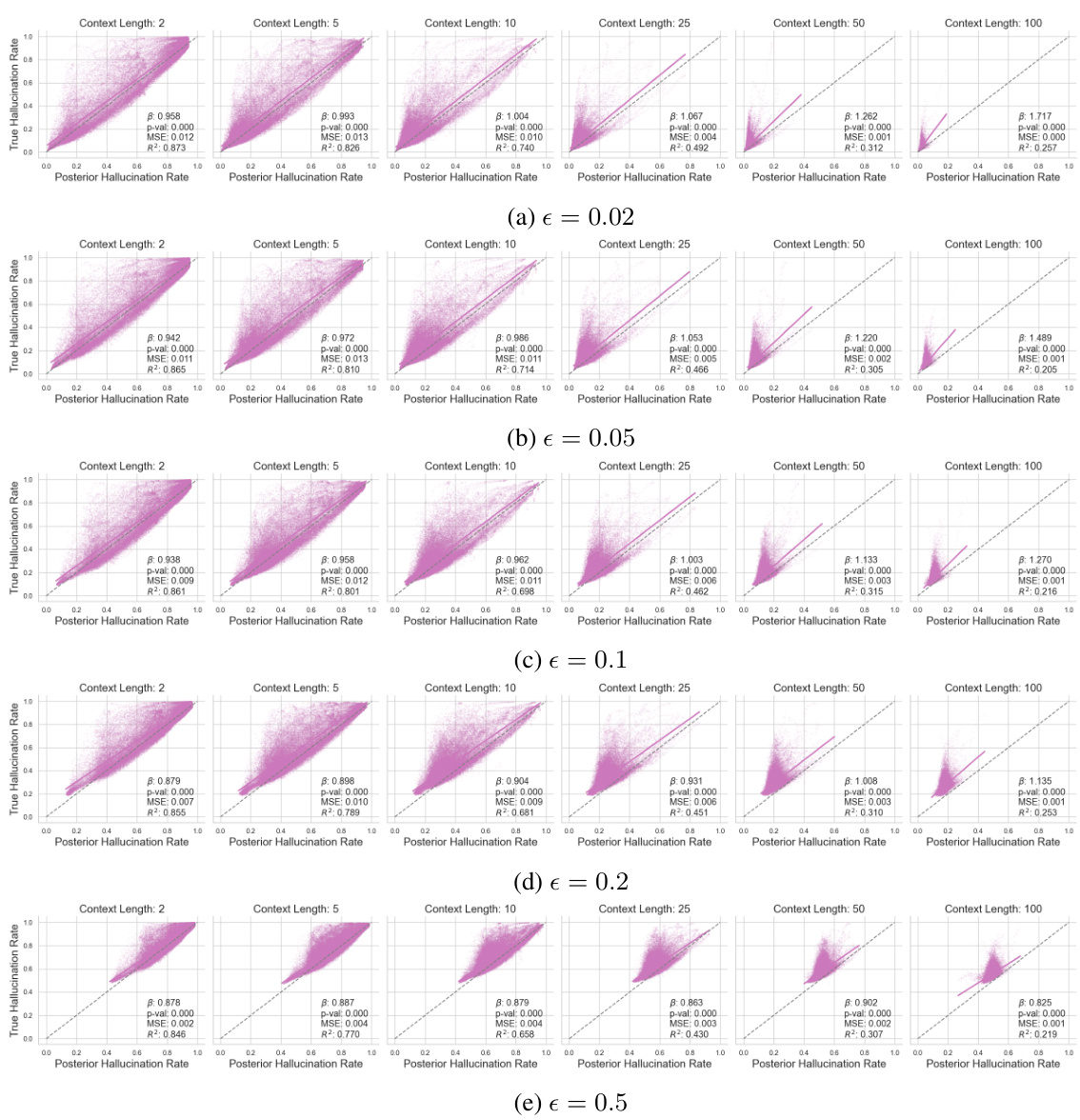
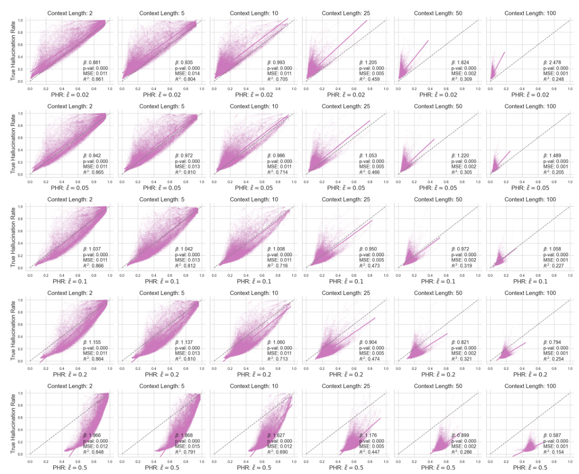
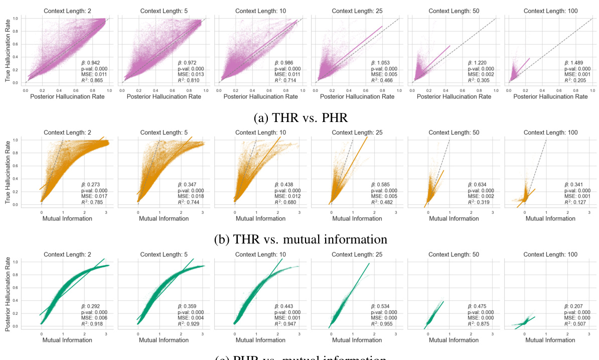
This figure displays the results of a synthetic regression experiment, comparing the true hallucination rate (THR) and the posterior hallucination rate (PHR) estimator for different sizes of the in-context dataset (n). Panel (a) shows that THR and PHR decrease and track each other very closely as n increases. Panel (b) shows a scatter plot demonstrating the calibration of the PHR estimator, showing the PHR closely aligns with the THR across different sizes of the dataset, although the accuracy decreases as context length increases.

This figure shows the results of a synthetic regression experiment. The top row (n=2 and n=100) shows the data generated by the neural process model and the true and estimated (1-ε) likely sets. The blue region shows the true (1-ε) likely set, while the purple shows the estimated set based on a small number of observations. The bottom row shows the true hallucination rate (THR) and the posterior hallucination rate (PHR). The plots illustrate how the PHR (estimated hallucination rate) aligns with the THR (true hallucination rate) and how both metrics improve (reduce) as more contextual examples are given.

This figure shows the relationship between the True Hallucination Rate (THR) and the Posterior Hallucination Rate (PHR) for synthetic regression data with varying numbers of context examples (n). Panel (a) demonstrates that as the number of context examples increases, both THR and PHR decrease, showing a strong positive correlation. Panel (b) displays a calibration plot, where each point represents the PHR and THR for a single instance. The closer the points are to the diagonal line (x=y), the better the PHR’s accuracy as a predictor of THR. While the PHR is generally a good estimator, the figure shows that its accuracy decreases as the context length increases.

This figure shows the results of a synthetic regression experiment comparing the posterior hallucination rate (PHR) and the true hallucination rate (THR) for different dataset sizes (n=2 and n=100). The blue shaded regions represent the (1-ε)-likely sets for the true data-generating process (THR), calculated using the true underlying model, while the purple regions show the (1-ε)-likely sets estimated by the CGM (PHR). As the number of data points increases from n=2 to n=100, the purple region converges toward the blue region, indicating improved accuracy of the CGM’s predictions. The plots clearly illustrate how the PHR (model estimate) becomes more accurate as the size of the training dataset increases, closely tracking the THR (true value).

This figure visualizes the results of a synthetic regression experiment. It compares the neural process’s generated outcomes for two different dataset sizes (n=2 and n=100). The blue shaded region represents the (1-ε)-likely set based on the true underlying data generating process, while the purple region shows the same set but conditioned on observed data. The panels on the right show the corresponding posterior hallucination rate (PHR) and true hallucination rate (THR) estimations. The plots visually demonstrate how the model’s uncertainty decreases as the amount of available context data increases.
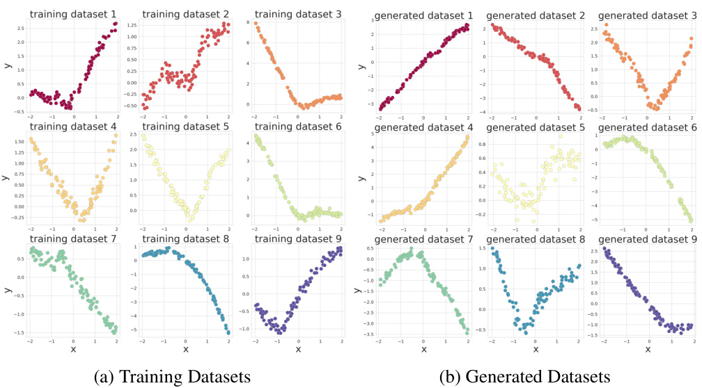
This figure shows the neural process’s generated outcomes for different dataset sizes (n=2 and n=100). The blue region represents the true (1-ε)-likely set based on the true underlying function, while the purple region shows the (1-ε)-likely set from the model’s perspective, conditioned on the observed data. The plots illustrate how the posterior hallucination rate (PHR) and the true hallucination rate (THR) change across the input domain (x) for each dataset size. This helps visualize the model’s uncertainty and how well the PHR approximates the THR as the dataset size increases.
This figure compares the true and estimated hallucination rates for a synthetic regression task. The top row shows the generated outcomes of a neural process model for two different dataset sizes (n=2 and n=100). The blue shaded area represents the true (1-ε)-likely set, meaning the range of values with at least a 1-ε probability under the true data generating distribution. The purple shaded area represents the corresponding range based on the model’s posterior predictive distribution. The lower row of the figure illustrates the true hallucination rate (THR, in blue) and the estimated posterior hallucination rate (PHR, in purple) as a function of input x, for both dataset sizes. The figure aims to demonstrate that PHR is a good estimator for THR.

This figure shows a comparison of the true hallucination rate (THR) and the posterior hallucination rate (PHR) for different dataset sizes (n=2 and n=100). The blue shaded regions represent the (1-ε)-likely sets of the true generative model, while the purple regions represent the (1-ε)-likely sets of the model’s posterior predictive distribution. The plots show that as the dataset size increases, the model’s posterior predictive distribution becomes more aligned with the true distribution, reducing the rate of hallucinations.
This figure demonstrates the results of synthetic regression experiments with different numbers of data points (n=2 and n=100). The top row shows the generated outcomes (blue for true and purple for estimated). The bottom row shows the corresponding posterior hallucination rate (PHR) and true hallucination rate (THR) across the domain. The results show that PHR closely aligns with THR as the number of data points increases.

This figure shows the relationship between the true hallucination rate (THR) and the posterior hallucination rate (PHR) for synthetic regression data. Panel (a) shows that as the number of context examples (n) increases, both THR and PHR decrease, indicating that the PHR is a good estimator of the THR. Panel (b) further validates this by showing a strong correlation between the predicted PHR and actual THR. However, the accuracy of the PHR estimator decreases as the context length increases.
This figure shows the results of synthetic regression experiments comparing the posterior hallucination rate (PHR) and the true hallucination rate (THR). The top row shows the model’s generated outcomes for different dataset sizes (n=2 and n=100). The bottom row shows the PHR and THR curves across the domain. The blue region represents the true (1-ε)-likely set for each model, and the purple region represents the likely set based on the model’s prediction.
This figure shows a comparison between the true hallucination rate (THR) and the posterior hallucination rate (PHR) for a synthetic regression task. The left and right panels depict the neural process’s generated outcomes (with different numbers of training data points) and the corresponding (1-ε)-likely sets for true and estimated responses. The central panels show the THR and PHR across the input domain. The comparison illustrates how accurately the PHR estimates the THR for different sample sizes.

This figure shows the comparison between the true hallucination rate (THR) and the posterior hallucination rate (PHR) for different numbers of data points (n=2 and n=100). The blue region represents the (1-ε)-likely set based on the true generative model, while the purple region represents the (1-ε)-likely set based on the model’s predictions. The plots show that as the number of data points increases, the PHR becomes a better estimate of the THR, indicating that the model’s uncertainty decreases and its predictions become more accurate. This demonstrates the effectiveness of the proposed method for estimating hallucination rates.

This figure shows a comparison of the true hallucination rate (THR) and the posterior hallucination rate (PHR) for synthetic regression tasks. The top row shows the generated outcomes of a neural process model for two different dataset sizes (n=2 and n=100). The blue region represents the (1-ε)-likely set based on the true data generating process; the purple region shows the (1-ε)-likely set predicted by the model based on the observed data. The bottom row shows plots of the PHR and THR across the input domain (x). This visualization helps to understand how the model’s prediction uncertainty relates to the true uncertainty and how this relationship changes with the size of the training dataset.

This figure shows the comparison of the generated outcomes by the neural process model with the true and posterior hallucination rates, showing how the model’s uncertainty changes with the amount of data (n). The blue region represents the actual likely set of responses given the mechanism f*, while the purple region is generated by the model given the context data. The second and fourth panels show how the PHR and THR align with the actual (1-ε)-likely sets. As the number of data points (n) increases, the purple region becomes more aligned with the blue region, demonstrating that the posterior hallucination rate aligns well with the true hallucination rate.

This figure shows the results of a synthetic regression experiment. The top row shows the model’s generated outcomes for different dataset sizes (n=2 and n=100). The blue shaded region represents the true (1-ε)-likely set, which is the set of responses that are likely to be generated from the underlying true data distribution. The purple shaded region represents the likely set, when considering the context. The bottom row shows the posterior hallucination rate (PHR) and the true hallucination rate (THR) for the different dataset sizes. The PHR is the probability that the model will generate a response that is unlikely, given the context, whereas the THR is the probability that a hallucination will be generated, given the true data distribution.

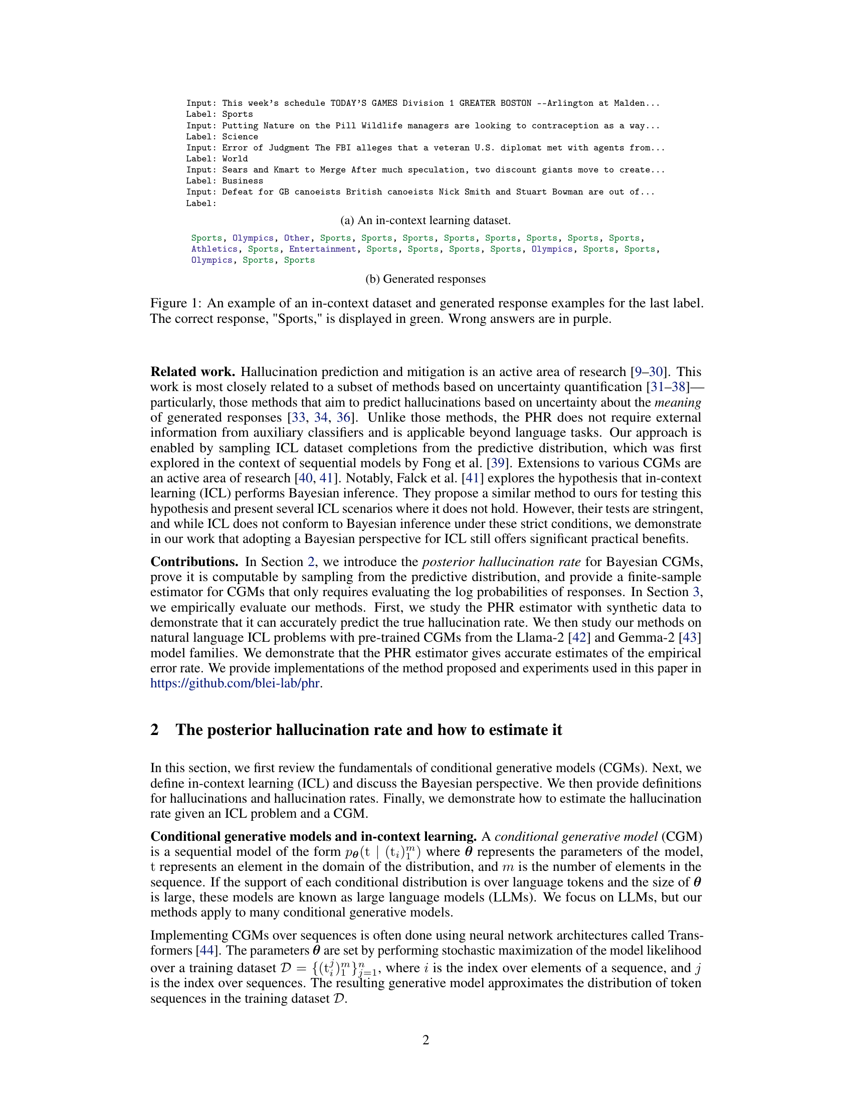
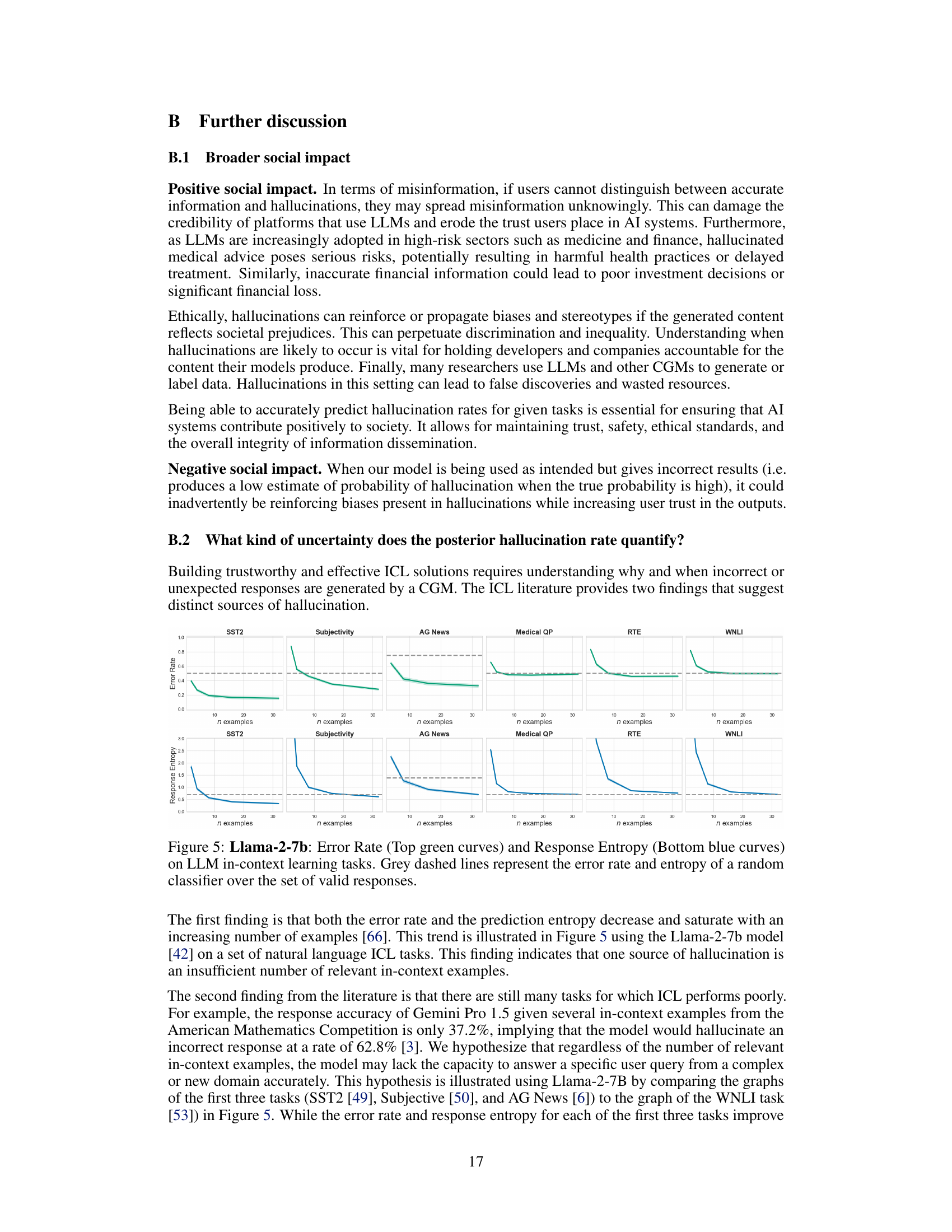
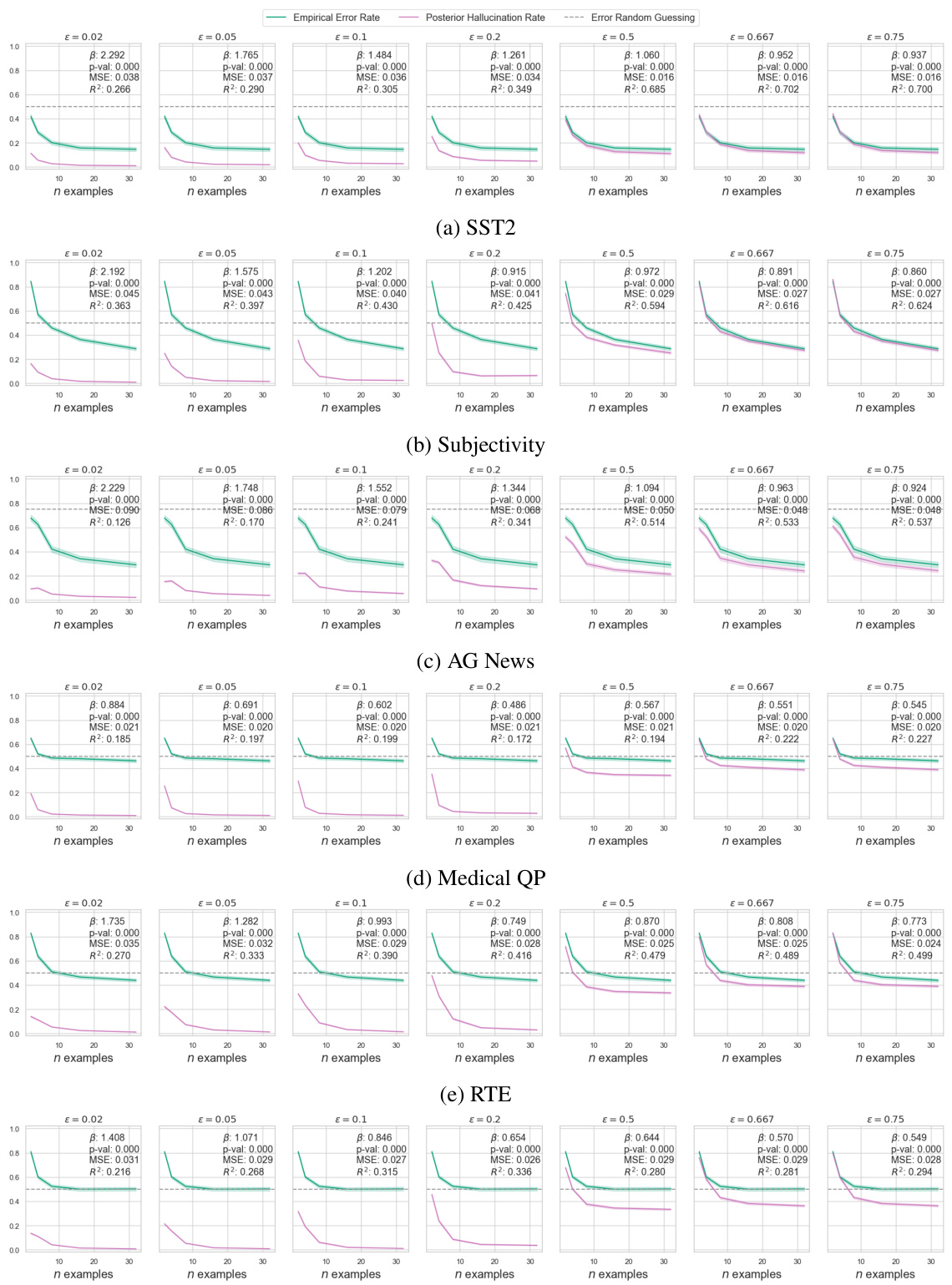
This figure shows the performance of Llama-2-7b on six different natural language in-context learning tasks. The top curves (green) show the model’s error rate in predicting the correct response, while the bottom curves (blue) show the predictive entropy. The grey dashed lines show the baseline error rate and entropy of a random classifier. The x-axis represents the number of in-context examples used, and the y-axis represents both the error rate and the predictive entropy. The figure illustrates how both the error rate and entropy decrease with more in-context examples, indicating improved model performance. However, the rate of improvement varies significantly across different tasks, highlighting the complexity of ICL in natural language.

This figure displays the results of synthetic regression experiments. The left and right panels in the top row show the neural process’s generated outcomes for datasets with 2 and 100 examples, respectively. The blue region represents the (1-ε)-likely set based on the true generative model, while the purple region is the likely set determined by the model, conditioned on the data. The bottom panels show the posterior hallucination rate (PHR) and the true hallucination rate (THR) calculated by the model.

This figure shows the comparison between the true hallucination rate (THR) and the posterior hallucination rate (PHR) for a synthetic regression task. The top row shows the neural process’s generated outcomes (model’s predictions) for datasets of size n=2 and n=100. The blue region represents the true likely set of outputs (based on the true underlying data generating process), while the purple region shows the model’s likely set of outputs (based on the model’s learned distribution). The bottom row shows the THR and PHR calculated across the range of input values (x). The graphs illustrate how increasing the dataset size (n) improves the model’s ability to predict likely outputs, resulting in a closer alignment between THR and PHR.

This figure shows the results of a synthetic regression experiment. The top row illustrates the model’s prediction for two different dataset sizes (n=2 and n=100). The blue shaded area shows the (1-ε)-likely set based on the true underlying data generating process (which is known in this synthetic setting). The purple area shows the model’s predicted (1-ε)-likely set given the observed data. The bottom row shows the posterior hallucination rate (PHR) and the true hallucination rate (THR) for the same datasets. The figure demonstrates that the PHR accurately estimates THR and that both decrease with increasing data size (n).
This figure shows the results of a synthetic regression experiment with different numbers of in-context examples. The top row shows the generated data for n=2 and n=100, with the blue region representing the true (1-ε)-likely set and the purple region representing the likely set conditioned on the observed data. The bottom row shows the corresponding posterior hallucination rate (PHR) and true hallucination rate (THR) curves across the x-domain. The plots show that, with increasing number of in-context examples, both the PHR and THR approach the ground truth.

This figure shows a comparison of the true hallucination rate (THR) and the posterior hallucination rate (PHR) for a synthetic regression task. The top row shows the generated data and the (1-ε)-likely sets for different numbers of data points (n=2 and n=100). The blue region represents the true (1-ε)-likely set based on the ground truth function, while the purple region represents the (1-ε)-likely set predicted by the model. The bottom row shows the PHR and THR plotted against the input values. This demonstrates how the PHR estimator accurately predicts the THR, especially with smaller dataset sizes.
Full paper#

