Label Delay in Online Continual Learning

m5CAnUui0Z

Botos Csaba et el.

TL;DR
#

Many real-world machine learning applications involve a time lag between data acquisition and label assignment, a phenomenon known as label delay. This delay significantly impacts the performance of online continual learning models which typically assume immediate label availability. Existing approaches like self-supervised learning and test-time adaptation struggle to compensate for this delay, often underperforming a naive method that simply trains on the delayed labeled data.

To address this challenge, this paper introduces a novel continual learning framework that explicitly models label delay and proposes a new method called Importance Weighted Memory Sampling (IWMS). IWMS effectively bridges the accuracy gap caused by label delay by strategically selecting and prioritizing memory samples that are highly similar to the newest unlabeled data. This ensures the model continuously adapts to evolving data distributions, improving its accuracy and robustness against significant label delays. Extensive experiments demonstrate that IWMS outperforms state-of-the-art approaches across multiple datasets and computational budget scenarios.

Key Takeaways
#

Why does it matter?
#

This paper is crucial for researchers in online continual learning as it addresses the often-overlooked challenge of label delay, offering novel solutions and insights into data utilization strategies for improved model accuracy and robustness in dynamic real-world scenarios. It highlights the limitations of existing approaches, opens avenues for developing computationally efficient methods, and fosters a deeper understanding of the impact of label delay on various learning paradigms.

Visual Insights
#

🔼 This figure illustrates the concept of label delay in continual learning. At each time step, new unlabeled data arrives, but the corresponding labels are delayed by a certain number of time steps (d). The figure shows how the model is evaluated on the newest unlabeled data but trained on both this data and the delayed labeled data. The colored images represent the delayed labeled data, while the grayscale images represent the current unlabeled data. The hourglass symbol next to the annotator represents the delay in getting labels.
read the caption
Figure 1: Illustration of label delay. This figure shows a typical Continual Learning (CL) setup with label delay due to annotation. At every time step t, the data stream Sx reveals a batch of unlabeled data {xt}, on which the model ftθ is evaluated (highlighted with green borders). The data is then sent to the annotator Sy who takes d time steps to provide the corresponding labels. Consequently, at time step t the batch of labels {yt−d} corresponding to the input data from d time steps before becomes available. The CL model can be trained using the delayed labeled data (shown in color) and the newest unlabeled data (shown in grayscale). In this example, the stream reveals three samples at each time step and the annotation delay is d = 2.

🔼 This table presents the accuracy scores obtained by the Naïve method on the Yearbook dataset. The rows represent the time ranges of the training data, and the columns represent the time ranges of the test data. Each cell in the table shows the accuracy of the Naïve method when trained on the training data and tested on the test data.
read the caption
Table 1: Accuracy matrix for Naïve method on Yearbook dataset.

In-depth insights
#

Label Delay Effects
#

The effects of label delay in online continual learning are significant and multifaceted. Simply increasing computational resources is insufficient to mitigate the negative impact on model performance. The core issue is the growing discrepancy between the distribution of the most recently observed (unlabeled) data and the older, labeled data used for training. State-of-the-art techniques like self-supervised learning and test-time adaptation fail to effectively bridge this accuracy gap, often underperforming a naive approach that solely utilizes the delayed labeled data. This highlights the critical need for methods explicitly designed to handle label delay, such as the importance weighted memory sampling technique, which prioritizes memory samples that closely resemble the newest unlabeled data. Effective solutions must go beyond increasing computational budget and cleverly manage the data used for training to bridge the performance gap between delayed and non-delayed scenarios.

IWMS Method
#

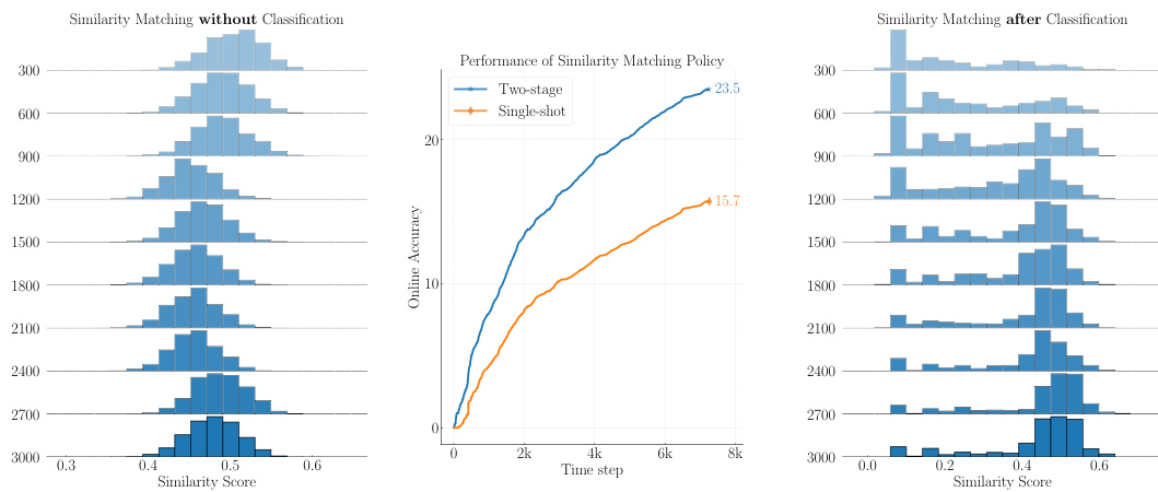
The Importance Weighted Memory Sampling (IWMS) method is a novel approach designed to address the challenges of label delay in online continual learning. IWMS cleverly bridges the accuracy gap caused by delayed labels by prioritizing memory samples that closely resemble the most recent unlabeled data. This is achieved through a two-stage process. First, the model predicts labels for the incoming unlabeled batch. Then, it selectively samples labeled data points from memory whose labels match the predicted labels and are most similar in feature space to the unlabeled data. This targeted sampling ensures the model adapts more effectively to the evolving data distribution despite the label delay, outperforming alternative semi-supervised, self-supervised and test-time adaptation approaches. The computational cost of IWMS remains manageable, only slightly increasing compared to the naive baseline, thus making it a practical and efficient solution for online continual learning in real-world scenarios with significant label delay.

Unsupervised Methods
#

The exploration of unsupervised methods in addressing label delay within online continual learning reveals both promising avenues and significant limitations. Self-Supervised Learning (SSL) approaches, while intuitively appealing due to their ability to leverage unlabeled data, surprisingly underperformed simpler baselines in many scenarios. This suggests that the computational overhead of SSL, even with carefully chosen methods, might outweigh the benefits in a time-sensitive, resource-constrained setting. Semi-Supervised Learning (SSL) methods, particularly pseudo-labeling, similarly exhibited mixed results, struggling to overcome the accuracy gap created by delayed labels. Test-Time Adaptation (TTA), designed to adapt models to new data distributions, also showed limited effectiveness, likely because of a mismatch between its inherent assumptions of data similarity and the real-world scenario of a dynamically changing data distribution over time. Overall, these findings highlight the challenge of efficiently integrating unlabeled data in continual learning settings with significant label delays. They emphasize that a naive approach of training only on delayed labeled data might remain surprisingly competitive. Future research should investigate more efficient and adaptable techniques for incorporating unlabeled data, perhaps focusing on methods tailored to address specific characteristics of delayed streams.

Computational Limits
#

The concept of ‘Computational Limits’ in the context of online continual learning with label delay is crucial. It highlights the inherent trade-off between model accuracy and the resources available for training. Simply increasing computational power may not resolve performance issues stemming from significant label delays. The paper emphasizes this constraint by normalizing computational budgets across different methods, preventing unfair comparisons. This focus on resource efficiency is vital as it promotes the development of practical algorithms suitable for real-world applications where computational resources are often limited. The authors investigate if increased computation can alleviate the accuracy drop caused by label delay, finding mixed results, thereby reinforcing the significance of efficient algorithms tailored to the label delay challenge. The ‘Computational Limits’ section underscores the need to consider resource constraints in evaluating different continual learning strategies and promotes the development of algorithms that are both accurate and computationally efficient.

Future Directions
#

Future research could explore several promising avenues. Developing more sophisticated methods for handling label delay is crucial, potentially involving advanced techniques in online learning or the integration of self-supervised learning methods to better utilize unlabeled data. Investigating the interaction between label delay, computational budget, and data characteristics across diverse continual learning scenarios would provide valuable insights into optimal resource allocation strategies. The impact of different data distributions and distribution shifts on the effectiveness of proposed methods requires further exploration to enhance the robustness of continual learning algorithms in real-world settings. Finally, extending the label delay framework to other continual learning paradigms (e.g., task-incremental learning) and exploring its implications for various application domains will broaden the impact and applicability of this important research area.

More visual insights
#

More on figures

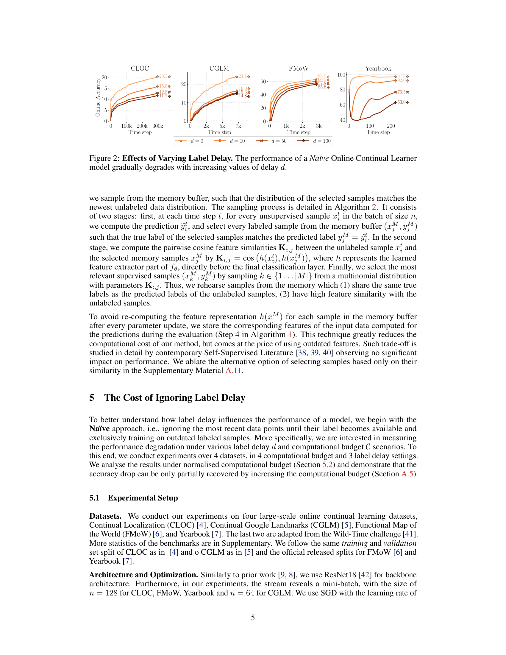
🔼 The figure shows the performance of a basic online continual learning model (Naïve) across four different datasets (CLOC, CGLM, FMoW, Yearbook) under varying label delays (d = 0, 10, 50, 100). The results demonstrate that as the label delay increases, the model’s accuracy consistently decreases. This is because the model is trained only on older, labeled data, while its performance is evaluated on more recent, unlabeled data. The gap in data distribution between training and evaluation leads to performance degradation. The severity of the accuracy drop is non-linear, meaning it is not the same across all datasets and varies with the length of the delay.
read the caption
Figure 2: Effects of Varying Label Delay. The performance of a Naïve Online Continual Learner model gradually degrades with increasing values of delay d.

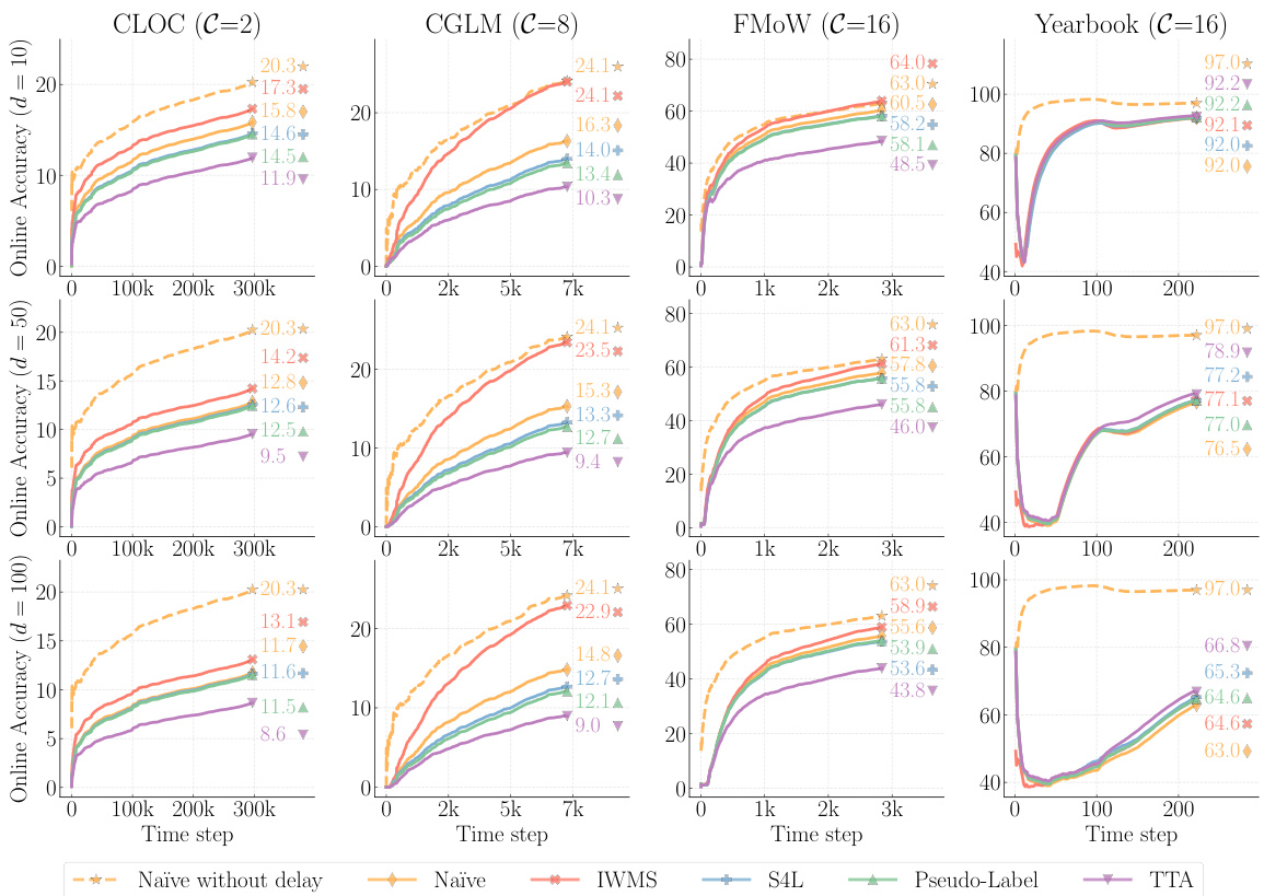
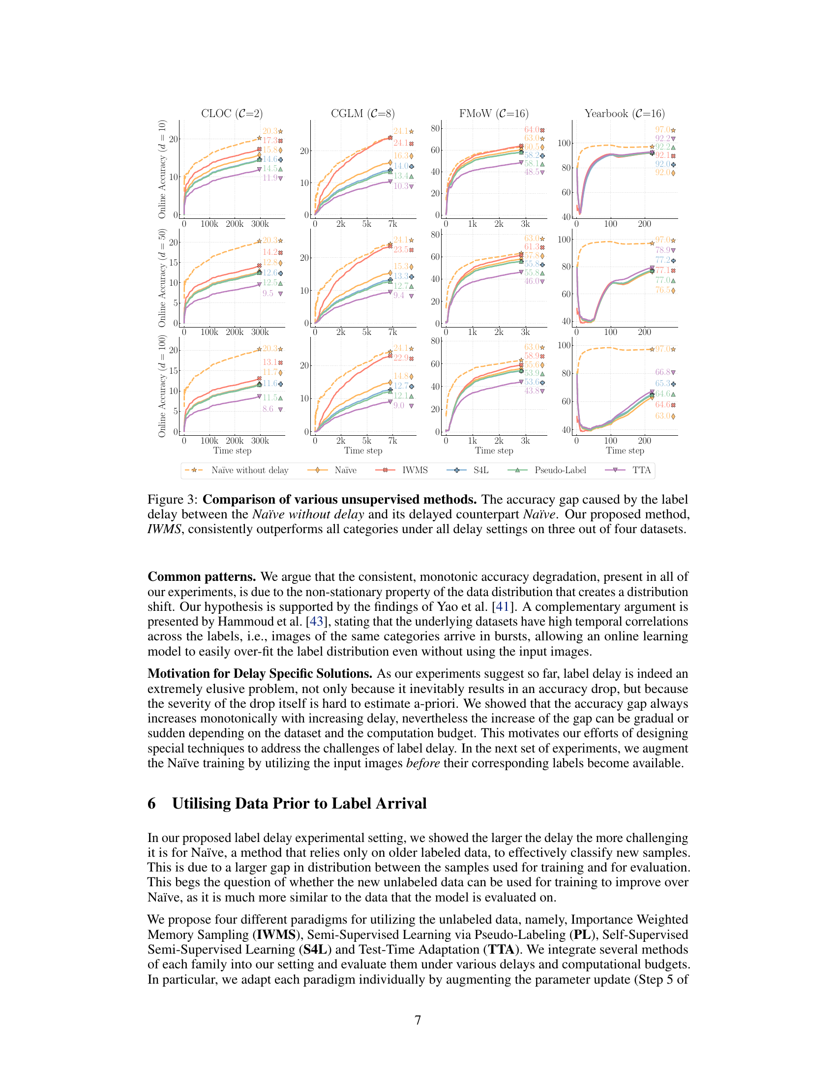
🔼 This figure compares the performance of different unsupervised methods (Naïve, IWMS, S4L, Pseudo-Label, TTA) in an online continual learning setting with varying label delays (10, 50, 100). It highlights the accuracy gap between a Naïve approach trained without delay and the same approach trained with delays. The results demonstrate that the proposed method, IWMS, significantly outperforms other methods across three out of four datasets, effectively mitigating the negative impact of label delay.
read the caption
Figure 3: Comparison of various unsupervised methods. The accuracy gap caused by the label delay between the Naïve without delay and its delayed counterpart Naïve. Our proposed method, IWMS, consistently outperforms all categories under all delay settings on three out of four datasets.

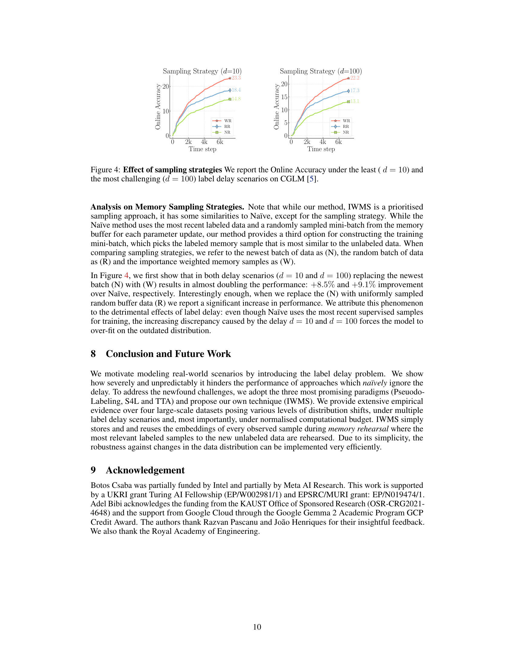
🔼 The figure shows the performance comparison of different sampling strategies (WR, RR, NR) in an online continual learning setting with label delay. WR represents Importance Weighted Memory Sampling, where samples from memory are selected based on similarity to the current unlabeled data. RR represents random sampling from memory, and NR represents only using the newest labeled data. The results are shown for two different label delay values (d=10 and d=100), demonstrating how IWMS outperforms the other strategies. The x-axis represents the timestep, and the y-axis represents the online accuracy.
read the caption
Figure 4: Effect of sampling strategies We report the Online Accuracy under the least (d = 10) and the most challenging (d = 100) label delay scenarios on CGLM [5].

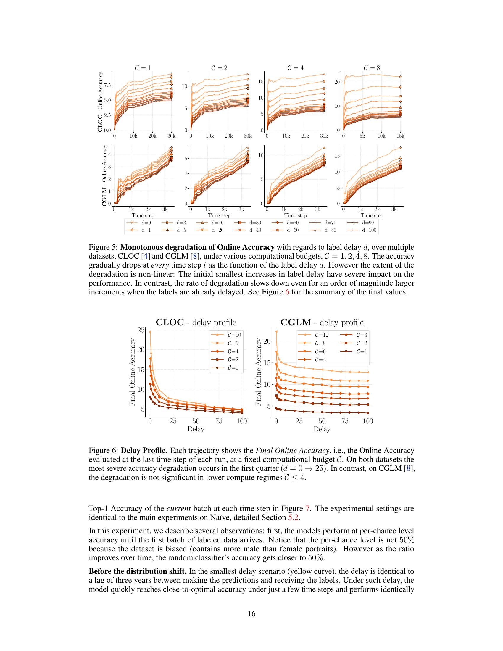
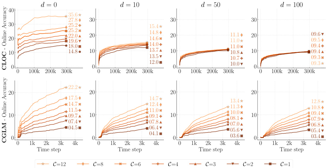
🔼 This figure shows how the online accuracy of a naive online continual learner degrades monotonically with increasing label delay (d) across various computational budgets (C). The top row displays results for the CLOC dataset, and the bottom for CGLM. Each line represents a different delay (d), showing how performance declines as the delay increases. The non-linearity of the degradation is emphasized; small initial delays cause significant accuracy drops, whereas the rate of decline slows down for larger delays. The figure highlights the substantial impact of even small label delays on model performance.
read the caption
Figure 5: Monotonous degradation of Online Accuracy with regards to label delay d, over multiple datasets, CLOC [4] and CGLM [8], under various computational budgets, C = 1, 2, 4, 8. The accuracy gradually drops at every time step t as the function of the label delay d. However the extent of the degradation is non-linear: The initial smallest increases in label delay have severe impact on the performance. In contrast, the rate of degradation slows down even for an order of magnitude larger increments when the labels are already delayed. See Figure 6 for the summary of the final values.

🔼 The figure shows the performance of a naive online continual learning model across four different datasets (CLOC, CGLM, FMoW, Yearbook) with varying label delays (d = 0, 10, 50, 100). The results demonstrate that the model’s accuracy consistently decreases as the label delay increases. This highlights the negative impact of label delay on the model’s ability to learn effectively from the data.
read the caption
Figure 2: Effects of Varying Label Delay. The performance of a Naïve Online Continual Learner model gradually degrades with increasing values of delay d.

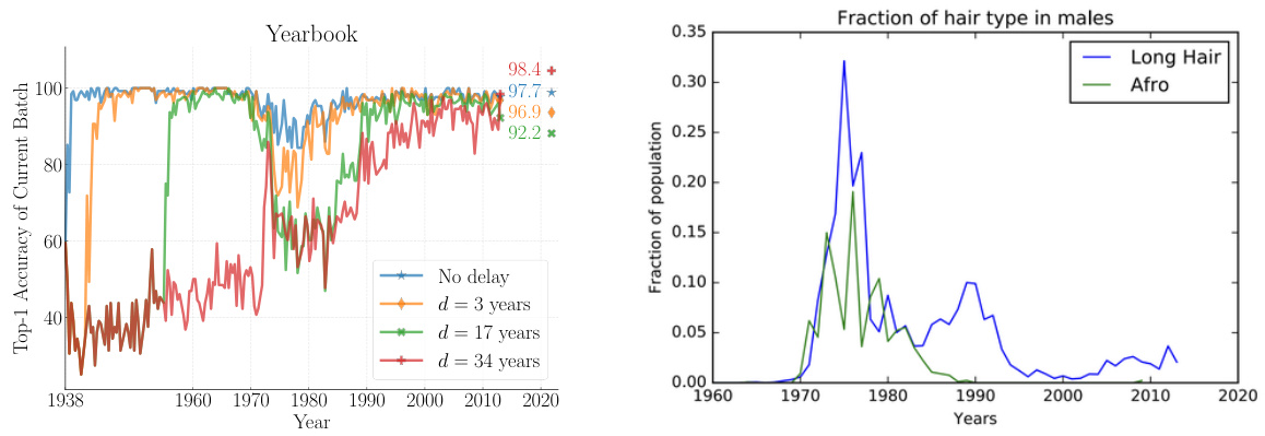
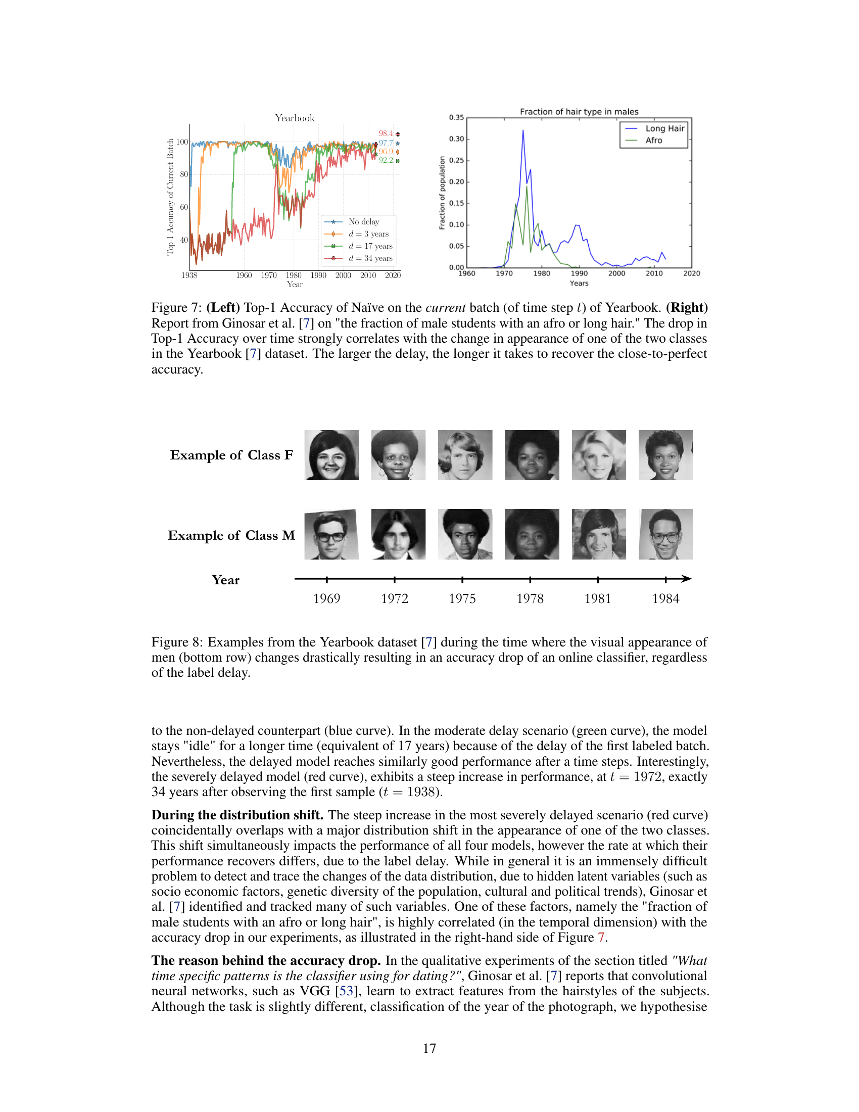
🔼 This figure shows two plots. The left plot shows the Top-1 accuracy of the Naïve model on the Yearbook dataset over time. It displays how the accuracy fluctuates, with a significant drop occurring around the 1970s. The different colored lines represent different levels of label delay (0, 3, 17, and 34 years). The longer the delay, the more prolonged the recovery time is after the accuracy drop. The right plot shows the fraction of male students with either long hair or afros over time, taken from Ginosar et al. [7]. This data highlights a major change in hairstyle trends during the 1970s, which is strongly correlated with the accuracy drop observed in the left plot. This demonstrates how shifts in the data distribution, reflected in changing fashion trends, can impact the performance of the Naïve model, especially with label delays.
read the caption
Figure 7: (Left) Top-1 Accuracy of Naïve on the current batch (of time step t) of Yearbook. (Right) Report from Ginosar et al. [7] on 'the fraction of male students with an afro or long hair.' The drop in Top-1 Accuracy over time strongly correlates with the change in appearance of one of the two classes in the Yearbook [7] dataset. The larger the delay, the longer it takes to recover the close-to-perfect accuracy.

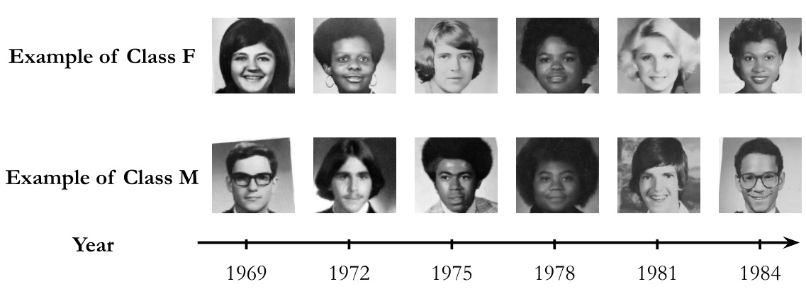
🔼 This figure shows example images from the Yearbook dataset to illustrate the drastic visual changes in men’s appearance over time. These changes in appearance correlate with drops in the accuracy of online classifiers, irrespective of the label delay. The top row shows examples of images classified as female, while the bottom row shows examples of images classified as male. The images are arranged chronologically by year, progressing from 1969 to 1984.
read the caption
Figure 8: Examples from the Yearbook dataset [7] during the time where the visual appearance of men (bottom row) changes drastically resulting in an accuracy drop of an online classifier, regardless of the label delay.

🔼 This figure compares the performance of several unsupervised methods (IWMS, S4L, Pseudo-Labeling, TTA) for online continual learning with varying label delays (d = 10, 50, 100) across four datasets (CLOC, CGLM, FMoW, Yearbook). It highlights the accuracy gap between a naïve approach trained only on delayed labeled data and the same approach without delay. The results demonstrate that IWMS consistently outperforms other methods across different delay settings and datasets, effectively bridging the accuracy gap caused by label delay.
read the caption
Figure 3: Comparison of various unsupervised methods. The accuracy gap caused by the label delay between the Naïve without delay and its delayed counterpart Naïve. Our proposed method, IWMS, consistently outperforms all categories under all delay settings on three out of four datasets.

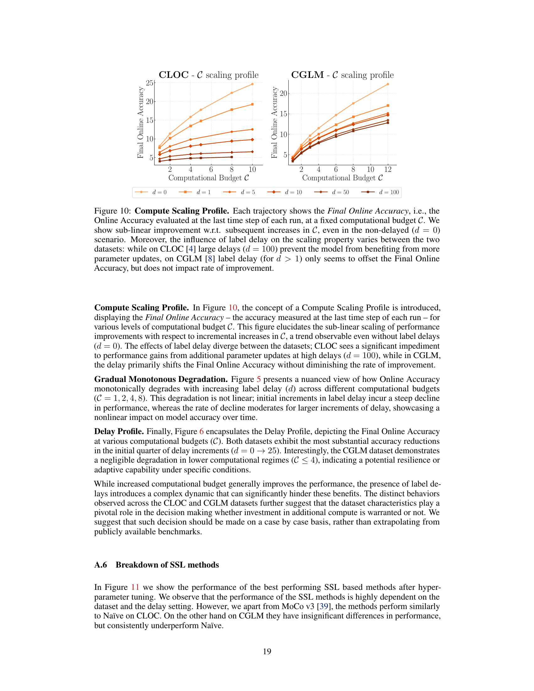
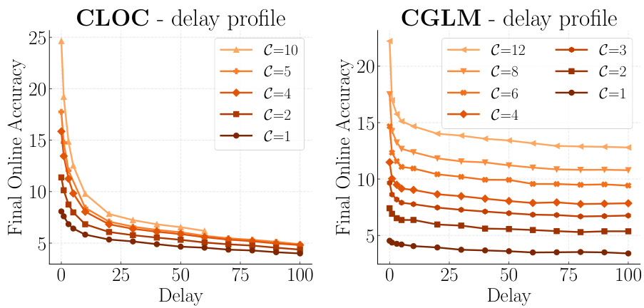
🔼 This figure shows the relationship between computational budget and online accuracy for two datasets (CLOC and CGLM) under various label delays. It demonstrates sub-linear returns on increasing computational budget, meaning that adding more computational resources yields progressively smaller accuracy gains. The effect of label delay also differs between datasets; on CLOC, large delays hinder the benefits of increasing the budget, while on CGLM, delays primarily shift the accuracy without significantly affecting improvement rates.
read the caption
Figure 10: Compute Scaling Profile. Each trajectory shows the Final Online Accuracy, i.e., the Online Accuracy evaluated at the last time step of each run, at a fixed computational budget C. We show sub-linear improvement w.r.t. subsequent increases in C, even in the non-delayed (d = 0) scenario. Moreover, the influence of label delay on the scaling property varies between the two datasets: while on CLOC [4] large delays (d = 100) prevent the model from benefiting from more parameter updates, on CGLM [8] label delay (for d > 1) only seems to offset the Final Online Accuracy, but does not impact rate of improvement.

🔼 This figure compares the performance of different unsupervised methods (Naïve, IWMS, S4L, Pseudo-Label, and TTA) in an online continual learning setting with varying label delays. It visualizes the accuracy of each method across four datasets (CLOC, CGLM, FMoW, and Yearbook) for different levels of delay. The results demonstrate that IWMS effectively mitigates the negative effects of label delays, consistently outperforming other methods on three out of the four datasets.
read the caption
Figure 3: Comparison of various unsupervised methods. The accuracy gap caused by the label delay between the Naïve without delay and its delayed counterpart Naïve. Our proposed method, IWMS, consistently outperforms all categories under all delay settings on three out of four datasets.

🔼 This figure compares the performance of different unsupervised methods for handling label delay in online continual learning. The methods compared include a naive approach (Naïve) that ignores unlabeled data, several state-of-the-art self-supervised, semi-supervised, and test-time adaptation techniques, and the authors’ proposed Importance Weighted Memory Sampling (IWMS) method. The results are shown across various delay scenarios and datasets, demonstrating that IWMS consistently outperforms other methods in bridging the accuracy gap introduced by label delay.
read the caption
Figure 3: Comparison of various unsupervised methods. The accuracy gap caused by the label delay between the Naïve without delay and its delayed counterpart Naïve. Our proposed method, IWMS, consistently outperforms all categories under all delay settings on three out of four datasets.

🔼 This figure compares the performance of different unsupervised methods for handling label delay in online continual learning. The x-axis represents the time step, and the y-axis shows the online accuracy. The figure shows that a naive approach, which only uses delayed labeled data, performs poorly as the label delay increases. The figure also shows that several state-of-the-art methods, such as self-supervised learning and test-time adaptation, fail to improve upon the naive approach. In contrast, the proposed method, Importance Weighted Memory Sampling (IWMS), consistently outperforms all other methods across different datasets and delay settings.
read the caption
Figure 3: Comparison of various unsupervised methods. The accuracy gap caused by the label delay between the Naïve without delay and its delayed counterpart Naïve. Our proposed method, IWMS, consistently outperforms all categories under all delay settings on three out of four datasets.

🔼 This figure compares the performance of several unsupervised methods for continual learning with label delay. It shows how the accuracy of a naive approach that only uses delayed labels degrades significantly with increasing delay. In contrast, the proposed Importance Weighted Memory Sampling (IWMS) method substantially reduces this accuracy gap across different datasets and delay levels, outperforming other unsupervised methods (Self-Supervised Learning (S4L), Pseudo-Labeling (PL), and Test-Time Adaptation (TTA)).
read the caption
Figure 3: Comparison of various unsupervised methods. The accuracy gap caused by the label delay between the Naïve without delay and its delayed counterpart Naïve. Our proposed method, IWMS, consistently outperforms all categories under all delay settings on three out of four datasets.

🔼 This figure compares the performance of different unsupervised methods (Naïve, IWMS, S4L, Pseudo-Labeling, TTA) for online continual learning under varying label delays (d = 10, 50, 100). The results are shown across four datasets (CLOC, CGLM, FMoW, Yearbook). The key takeaway is that the proposed method, IWMS, consistently outperforms other methods in mitigating the negative impact of label delay, especially on three out of four datasets.
read the caption
Figure 3: Comparison of various unsupervised methods. The accuracy gap caused by the label delay between the Naïve without delay and its delayed counterpart Naïve. Our proposed method, IWMS, consistently outperforms all categories under all delay settings on three out of four datasets.

🔼 This figure illustrates the concept of label delay in continual learning. Unlabeled data arrives at each time step (t), but the corresponding labels are delayed by a fixed number of steps (d). The figure visually shows how the model receives both unlabeled data from the current time step and delayed labels from previous time steps. This setup highlights the challenge of continual learning when labels are not immediately available.
read the caption
Figure 1: Illustration of label delay. This figure shows a typical Continual Learning (CL) setup with label delay due to annotation. At every time step t, the data stream Sx reveals a batch of unlabeled data {xt}, on which the model ft is evaluated (highlighted with green borders). The data is then sent to the annotator Sy who takes d time steps to provide the corresponding labels. Consequently, at time step t the batch of labels {yt−d} corresponding to the input data from d time steps before becomes available. The CL model can be trained using the delayed labeled data (shown in color) and the newest unlabeled data (shown in grayscale). In this example, the stream reveals three samples at each time step and the annotation delay is d = 2.

🔼 The figure illustrates the experimental setup used in the paper to investigate the impact of label delay on online continual learning. It shows how the arrival of new data and its corresponding labels is separated by a delay. The purple blocks represent labeled data used in the Naïve method, while the gray blocks indicate unlabeled data. The three paradigms explored to mitigate the impact of label delay are Self-Supervised Learning, Test-Time Adaptation, and Importance Weighted Memory Sampling.
read the caption
Figure 17: Experimental setup: in our experiments we show how increased label delay affects the Naïve approach that simply just waits for the labels to arrive. To counter the performance degradation we evaluate three paradigms (Self-Supervised Learning, Test-Time Adaptation, Importance Weighted Memory Sampling) that can augment the Naïve method by utilizing the newer, unsupervised data.

🔼 This figure compares the performance of several unsupervised methods for handling label delay in online continual learning across four datasets: CLOC, CGLM, FMoW, and Yearbook. The x-axis represents the time steps, and the y-axis shows the online accuracy. The figure highlights the accuracy gap between a naïve method trained without label delay and the same method with label delay (Naïve). It shows that the proposed method, IWMS, significantly outperforms other unsupervised methods like self-supervised learning, semi-supervised learning, and test-time adaptation in mitigating the negative impact of label delay on accuracy, particularly in three of the four datasets shown.
read the caption
Figure 3: Comparison of various unsupervised methods. The accuracy gap caused by the label delay between the Naïve without delay and its delayed counterpart Naïve. Our proposed method, IWMS, consistently outperforms all categories under all delay settings on three out of four datasets.

🔼 This figure compares the performance of several unsupervised methods in an online continual learning setting with label delay. The methods compared are Naïve (using only delayed labels), Naïve without delay (a baseline with no delay), Importance Weighted Memory Sampling (IWMS - the proposed method), Self-Supervised Learning (S4L), and Test-Time Adaptation (TTA). The results are shown for four datasets (CLOC, CGLM, FMoW, Yearbook) across three levels of label delay (10, 50, 100 time steps). The key finding is that IWMS consistently outperforms all other methods across three of the four datasets, demonstrating its effectiveness in mitigating the accuracy loss due to label delay.
read the caption
Figure 3: Comparison of various unsupervised methods. The accuracy gap caused by the label delay between the Naïve without delay and its delayed counterpart Naïve. Our proposed method, IWMS, consistently outperforms all categories under all delay settings on three out of four datasets.

🔼 This figure shows how the performance of a simple online continual learning model (Naïve) is affected by varying the label delay (d). The x-axis represents the time step in the learning process, while the y-axis shows the accuracy. Multiple lines are shown, each corresponding to a different value of d (the label delay). As d increases, the final accuracy of the model consistently decreases, illustrating the negative impact of label delay on continual learning.
read the caption
Figure 2: Effects of Varying Label Delay. The performance of a Naïve Online Continual Learner model gradually degrades with increasing values of delay d.