↗ OpenReview ↗ NeurIPS Homepage ↗ Chat
TL;DR#
Calibrating computer models is crucial in many scientific fields but often requires numerous computationally expensive simulations. Existing methods mostly reuse existing designs, potentially missing informative correlations and wasting resources. This is particularly problematic in complex applications with high simulation costs.
This research presents BACON, a novel data-efficient algorithm that addresses this issue. By adopting a Bayesian adaptive experimental design approach, BACON jointly estimates parameters and optimal designs to maximize information gain at each step. This batch-sequential process uses Gaussian processes to effectively model simulations and correlate them with real data. Experiments across synthetic and real datasets showcase BACON’s superiority in terms of computational savings and estimation accuracy compared to existing approaches.
Key Takeaways#
Why does it matter?#
This paper is crucial for researchers in Bayesian optimization and experimental design. It offers a novel, data-efficient algorithm for calibrating computer models, particularly valuable when simulations are computationally expensive. The joint optimization of designs and calibration parameters, along with the use of Gaussian processes, presents significant improvements over existing methods. This work opens avenues for more efficient simulations in various fields, from climate modeling to robotics, impacting both theory and applications.
Visual Insights#

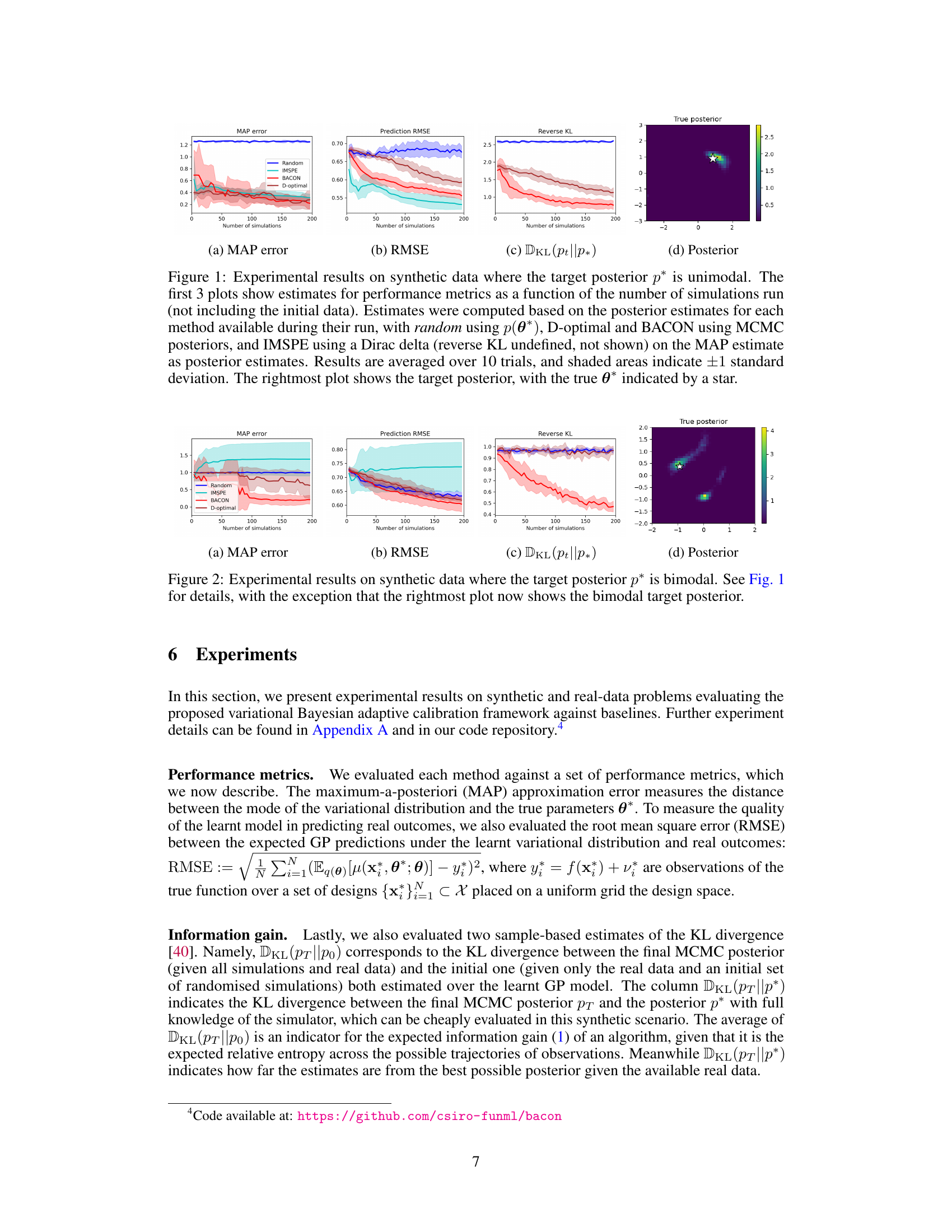
This figure displays the results of an experiment on synthetic unimodal data, comparing four methods: random search, IMSPE, BACON, and D-optimal. Three performance metrics (MAP error, RMSE, and Reverse KL divergence) are plotted against the number of simulations. The plots show that BACON outperforms the other methods in terms of reducing the MAP error and KL divergence, indicating it’s more effective at estimating the target posterior. The RMSE plots indicate that IMSPE is the best performer among the methods at predicting the real outcomes.

This table presents the results of experiments conducted on a 2+2D synthetic problem. The experiments compare the performance of different calibration methods after 50 iterations. The results are reported as the KL divergence between the final posterior and the initial (prior) posterior, and the KL divergence between the final posterior and the true posterior (given complete knowledge of the simulator). Lower KL divergence to the true posterior indicates better performance. The results are averages and standard deviations from 10 independent runs of each algorithm.
In-depth insights#
Adaptive Calibration#
Adaptive calibration techniques address the limitations of traditional calibration methods by iteratively refining model parameters based on observed data. Unlike static calibration, which assumes fixed parameter values, adaptive calibration dynamically updates these parameters as new information becomes available. This iterative process allows the model to better reflect the underlying system dynamics and improve its predictive accuracy over time. A key aspect of adaptive calibration is the selection of informative data points. Efficiently choosing when and where to gather additional data is crucial, as excessive data collection can be costly and time-consuming. Bayesian optimization and other experimental design techniques are often employed to guide this data acquisition, maximizing the information gained at each iteration. The effectiveness of adaptive calibration depends on various factors, including the complexity of the system, the quality of the initial model, and the effectiveness of the data selection strategy. Successful implementations often involve integrating sophisticated statistical methods with efficient computational algorithms. Moreover, there are opportunities to explore the use of advanced machine learning models within adaptive calibration frameworks, potentially enabling the automation and acceleration of the entire calibration process. However, challenges remain in addressing scalability and robustness issues as the complexity of the model and the size of the datasets increase.
Bayesian Approach#
A Bayesian approach to calibration is advantageous because it explicitly incorporates prior knowledge and uncertainty. This contrasts with frequentist methods that rely solely on observed data. By using Bayesian inference, we can update our beliefs about model parameters in light of new evidence, leading to more robust and accurate calibrations. The approach facilitates a principled way to quantify uncertainty in model predictions. A strength of Bayesian calibration is the natural integration with experimental design, which allows for adaptive optimization and efficient use of simulations. In Bayesian optimal experimental design, we iteratively select new experiments based on the expected information gain, ensuring maximum value from each run. This sequential approach is particularly useful for computationally expensive simulations. A limitation is the computational demands, especially for complex models and large datasets; however, methods like variational inference or sparse Gaussian processes can mitigate this. The Bayesian framework offers powerful tools for rigorous and principled calibration, potentially enhancing the reliability of scientific and engineering models.
Optimal Design#
Optimal experimental design is a crucial aspect of the research, focusing on efficiently using limited resources. The core idea is to strategically select simulations that maximize the information gained about unknown parameters. The approach moves beyond passively using existing data and actively shapes the experiment’s course. This involves sophisticated methods for jointly estimating posterior distributions and identifying optimal designs, often through maximizing a variational lower bound on expected information gain. Gaussian processes are used to model both the simulator and the uncertainty, allowing for correlations between simulations and data. The goal is to minimize the number of expensive simulations while achieving high-quality parameter estimates. This adaptive strategy, in contrast to fixed-design methods, dramatically improves efficiency by focusing computational effort where it yields the most information.
Gaussian Processes#
The application of Gaussian processes (GPs) in this research paper is multifaceted and crucial. GPs are employed as emulators to model the complex computer simulations, capturing uncertainty inherent in the simulator’s output. This probabilistic treatment is vital for handling the expense and uncertainty involved in running the simulations. The choice of GPs allows for correlation between simulation results and their corresponding inputs, and observed data. This correlation is especially significant when addressing limited data scenarios, offering a way to infer information even when simulation runs are restricted. By modeling both the simulations and observed data as samples from GPs, the paper’s approach naturally incorporates uncertainty estimation, a key aspect in Bayesian calibration frameworks. This use of GPs is essential to the paper’s contribution, providing a robust and flexible tool to tackle the challenges of data scarcity and computational cost in complex simulations.
Future Work#
The paper’s ‘Future Work’ section would ideally explore several avenues. Addressing the scalability limitations imposed by the cubic complexity of exact inference in Gaussian processes (GPs) is crucial. Exploring the use of scalable sparse GP methods or alternative approximation techniques to handle large datasets would significantly enhance the practical applicability of the proposed approach. Another important direction would involve investigating alternative variational families beyond the chosen conditional normalizing flows. This exploration could lead to improved performance in diverse scenarios, particularly with multimodal posteriors. Finally, extending the framework to handle multi-output observations and more complex simulator models would strengthen its generality and applicability to a broader spectrum of real-world problems. This would involve adapting the information-theoretic framework and employing multi-output GP models. Additionally, a comparison to alternative active learning strategies within the Bayesian calibration context would further refine understanding of the approach’s strengths and limitations.
More visual insights#
More on figures

This figure presents the experimental results of four different methods (Random, IMSPE, BACON, and D-optimal) on a unimodal synthetic dataset. It compares their performance in terms of MAP error (how close the estimated parameters are to the true parameters), prediction RMSE (how well the models predict real-world outcomes), and reverse KL divergence (how much information gain is achieved). The shaded regions represent the standard deviation across 10 independent trials. The rightmost plot visualizes the target posterior distribution to provide a context for interpreting the results.

This figure shows a soft robotics grasping experiment setup. It consists of three parts: (a) Platform, showing the automated experimentation platform with various shaped objects arranged on a table; (b) Real grasp, showcasing the robot gripper grasping one of the objects; (c) Simulation, illustrating a simulated version of the grasp using a soft materials simulator, with a visual representation of stress and strain. This experiment is used to calibrate the soft material simulator against real-world data.

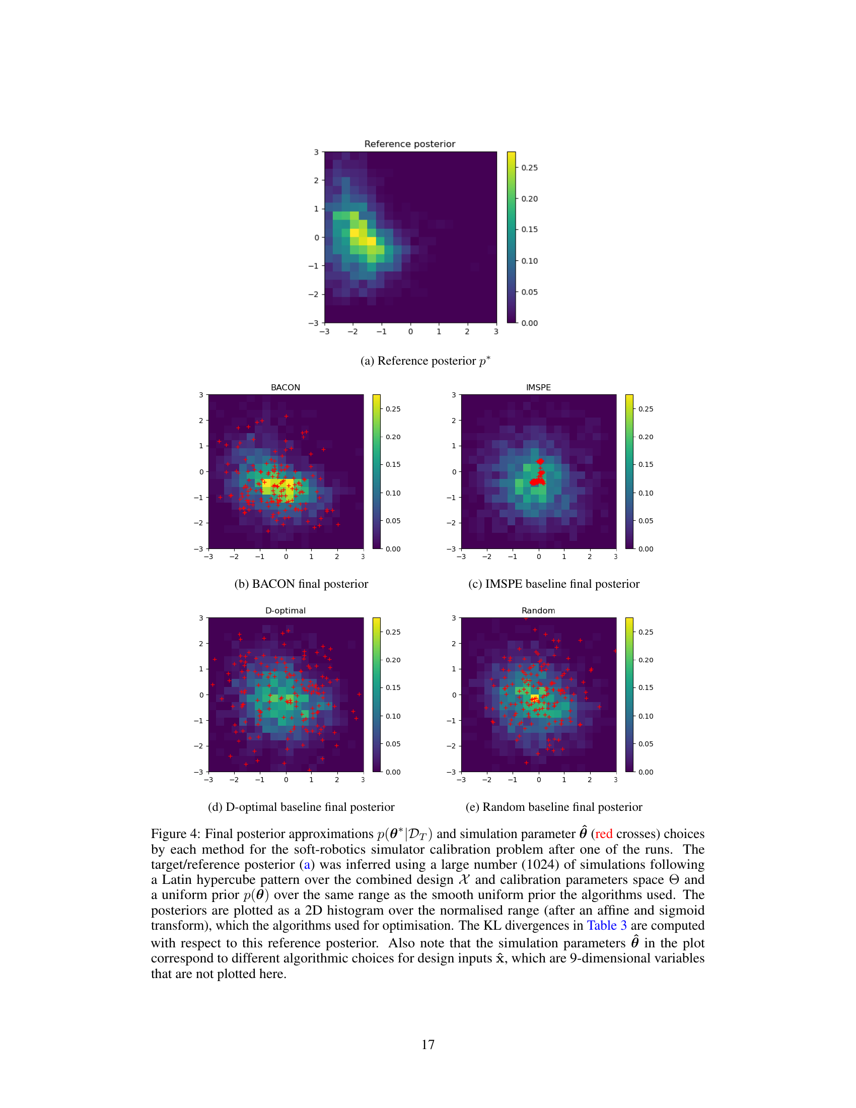
This figure compares the final posterior distributions obtained by different methods (BACON, IMSPE, D-optimal, Random) for a soft-robotics simulator calibration problem. The reference posterior is shown for comparison, obtained from a large number of simulations. The plots show 2D histograms of the posterior distributions, highlighting the differences in the accuracy and spread of the estimations obtained with each method.

This figure compares the final posterior distributions obtained by BACON, IMSPE, D-optimal, and random search methods for the soft-robotics grasping simulator calibration. The reference posterior is calculated using a large number of simulations to provide a ground truth. Each subplot shows the posterior distribution, with red crosses indicating the chosen simulation parameters. This illustrates how each method approximates the true posterior and its efficiency in exploring the parameter space.
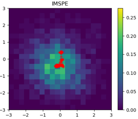
This figure compares the final posterior distributions obtained by different calibration methods for a soft-robotics simulator. The reference posterior is calculated using a large number of simulations. Each subplot shows a 2D histogram representing the final posterior for a particular method (BACON, IMSPE, D-optimal, Random), with red crosses indicating the chosen simulation parameters. The KL divergences (a measure of difference between probability distributions) are shown in Table 3.

This figure compares the final posterior approximations obtained by different calibration methods for a soft-robotics simulator. The reference posterior, calculated using a large number of simulations, is shown alongside the results for BACON, IMSPE, D-optimal, and random search. The plot highlights the differences in the posterior distributions and the locations of the sampled simulation parameters for each method.

This figure compares the final posterior distributions obtained by different calibration methods (BACON, IMSPE, D-optimal, Random) for a soft-robotics simulator calibration problem. The reference posterior, inferred using a large number of simulations, serves as a benchmark. Each plot visualizes the 2D marginal distribution of the two calibrated parameters, illustrating the performance of each method in terms of posterior approximation accuracy. The red crosses indicate the selected simulation parameters for each method during one of the algorithm runs. The differences in the posterior shapes reflect the strengths and weaknesses of each calibration approach.
More on tables
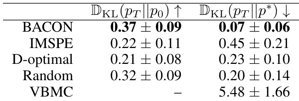
This table presents the results of the location finding problem experiment. It compares the performance of different algorithms (BACON, IMSPE, D-optimal, Random, and VBMC) after 30 iterations, using batches of 4 simulations at each iteration. The algorithms started with 20 real data points and 20 initial random simulations. The results show the average KL divergence between the final posterior and the initial posterior (DKL(PT||PO)) and the KL divergence between the final posterior and the true posterior (DKL(PT||P*)) across 10 independent runs. A higher DKL(PT||PO) indicates better information gain, while a lower DKL(PT||P*) suggests a closer approximation to the true posterior.
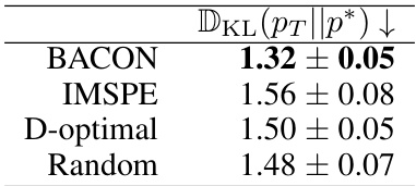
This table presents the results of a soft-robotics simulator calibration experiment. It compares four different methods (BACON, IMSPE, D-optimal, and Random) in terms of how well they approximate the true posterior distribution (p*) after 10 iterations with a batch size of 16. The lower the DKL(pT||p*) value, the better the approximation. The target posterior p* was determined using 1024 simulations for comparison.
Full paper#
