TL;DR#
Controlling complex physical systems is challenging due to limitations of classical methods and difficulties in optimizing long-term control sequences using deep learning. Existing methods often struggle with global optimization and generating controls that deviate from training data.
DiffPhyCon addresses these issues by using diffusion models for energy optimization across entire trajectories and control sequences. This approach facilitates global optimization and plans near-optimal sequences, even those deviating from training data, as shown by experiments on Burgers’ equation, jellyfish movement, and smoke control. The method’s superiority is demonstrated by its superior performance compared to existing approaches and the release of a new benchmark jellyfish dataset makes it a valuable contribution to the field.
Key Takeaways#
Why does it matter?#
This paper is crucial for researchers working on complex physical system control. It presents DiffPhyCon, a novel generative method that outperforms existing techniques, opening avenues for exploring near-optimal control sequences, especially those significantly deviating from training data distributions. The released dataset and code further enhance its impact, fostering advancements in this rapidly evolving field.
Visual Insights#

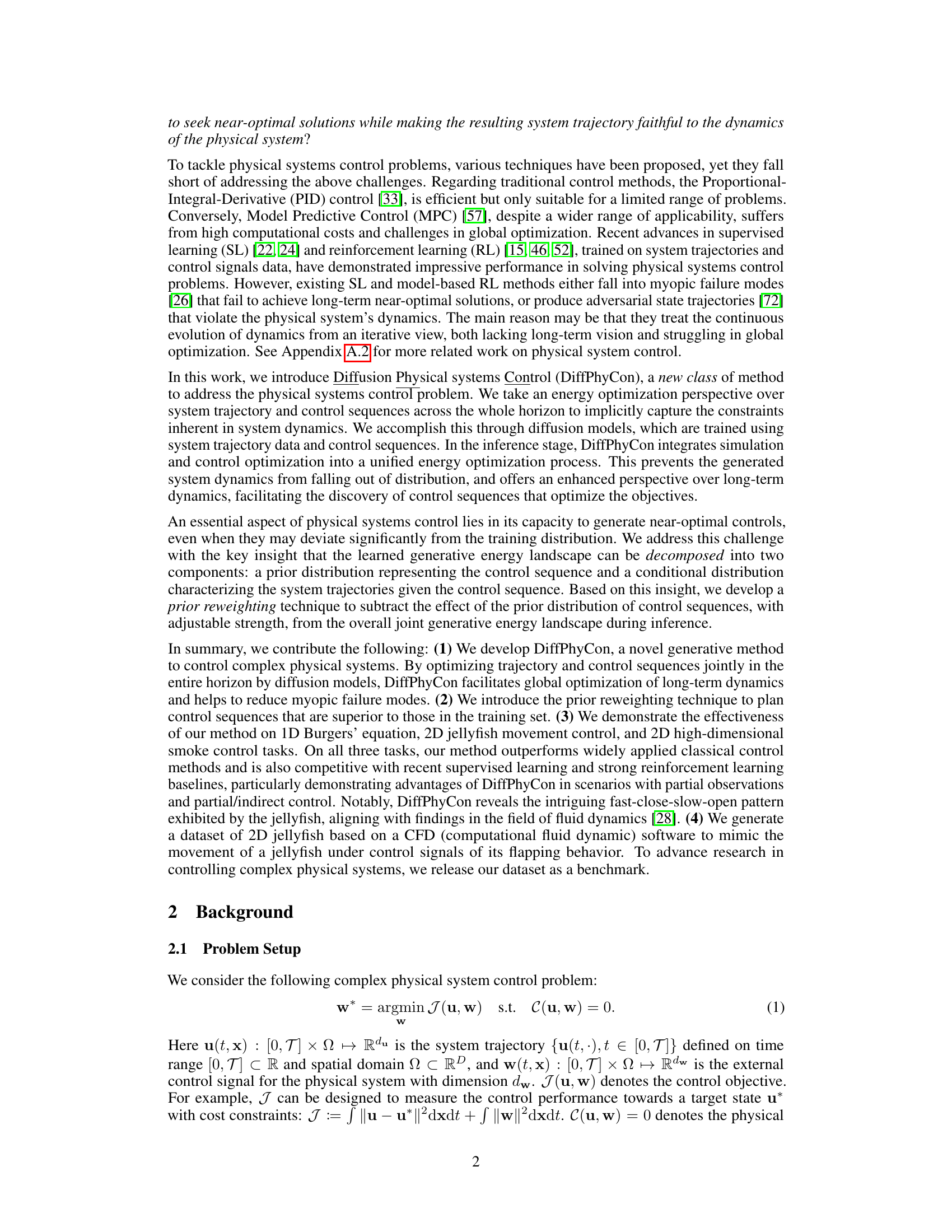
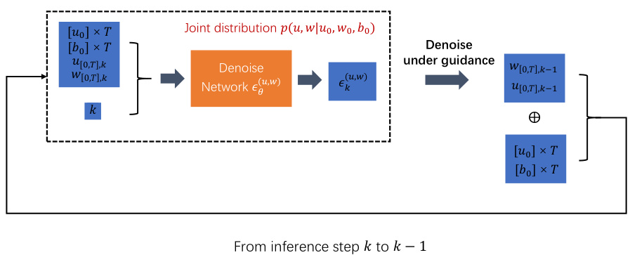
🔼 This figure illustrates the training, inference, and evaluation processes of the DiffPhyCon model. The training stage involves learning both the joint distribution of state trajectories and control sequences, and the prior distribution of control sequences. Inference uses this learned information, along with prior reweighting and guidance, to generate optimal control sequences. The evaluation stage assesses the performance of these generated sequences in controlling the physical system.
read the caption
Figure 1: Overview of DiffPhyCon. The figure depicts the training (top), inference (bottom left), and evaluation (bottom right) of DiffPhyCon. Orange and blue colors respectively represent models learning the joint distribution pe(u, w) and the prior distribution pf(w). Through prior reweighting and guidance, DiffPhyCon is capable of generating superior control sequences.

🔼 This table presents a summary of the characteristics of the jellyfish movement dataset used in the paper. It shows the number of training and testing trajectories, the resolution of the fluid features, the number of fluid features, and the length of each trajectory.
read the caption
Table 2: Jellyfish movement dataset outline.
In-depth insights#
Generative Control#
Generative control, in the context of complex physical systems, represents a paradigm shift from traditional control methodologies. Instead of relying solely on reactive feedback loops, generative models learn the underlying dynamics of the system, enabling proactive control strategies. This approach leverages the power of generative models to predict future states and optimize control sequences over the entire time horizon, avoiding the myopic decisions inherent in many reinforcement learning approaches. By minimizing a learned energy function that encompasses both generative and control objectives, generative control methods aim to discover near-optimal, globally consistent control sequences that are faithful to the system’s dynamics. Prior reweighting techniques further enhance the ability of these models to explore control sequences that deviate from the training data, potentially unveiling novel control patterns not observed during training. Overall, generative control offers a promising pathway towards solving complex physical control problems by combining the predictive power of generative models with optimization frameworks, leading to more robust and efficient control strategies.
Diffusion Models#
Diffusion models, a class of generative models, have emerged as a powerful tool for generating high-quality samples from complex data distributions. They function by gradually adding noise to data until it becomes pure noise, and then learning a reverse process to reconstruct the original data from the noise. This process is particularly effective because it enables the model to learn the data distribution by learning to remove noise, which is a more stable and tractable process than directly learning the data distribution. A key advantage is their ability to generate high-quality, diverse samples that are faithful to the original data distribution. This makes them suitable for various applications, including image generation, text generation, and more recently, control of physical systems. However, they can be computationally expensive to train, especially for high-dimensional data. Moreover, the exploration of their application in complex systems like controlling physical phenomena is a nascent field. Although early research shows promise in applications such as robotics and scientific simulations, further investigation into their strengths and limitations is necessary to fully understand their potential and overcome current challenges.
Prior Reweighting#
The core idea of ‘Prior Reweighting’ is to mitigate the undue influence of the training data distribution on the generation of control sequences. By decomposing the learned generative energy landscape into a prior distribution (representing control sequences) and a conditional distribution (representing system trajectories given controls), the method introduces a hyperparameter to reweight the prior. This allows exploration beyond the training distribution, leading to control sequences that may achieve near-optimal objectives despite deviating significantly from previously observed patterns. The reweighting technique effectively shifts the sampling focus towards less likely, yet potentially superior, regions of the energy landscape, thereby enhancing the model’s capacity for global optimization and enabling the discovery of novel control strategies. A key advantage is its adaptability, allowing for adjustable influence of the prior distribution during inference.
Benchmark Dataset#
A well-constructed benchmark dataset is crucial for evaluating and comparing different algorithms in the field of complex physical system control. The creation of such a dataset requires careful consideration of several factors: Firstly, the dataset must encompass a sufficiently wide range of scenarios to adequately test the capabilities of different algorithms. Secondly, it should include various levels of complexity and dimensionality to truly challenge state-of-the-art methods. The data must be of high quality to allow for accurate and reliable evaluations. This means proper data generation techniques, error handling, and thorough verification of the datasets’ fidelity to the physical phenomena under study are necessary. Furthermore, a well-documented dataset facilitates reproducibility in research and allows other researchers to build on previous work, creating a cumulative effect and accelerating progress in the field. Finally, the dataset should be publicly available, ideally with open licenses to maximize its impact and benefit the wider scientific community. The release of a high-quality benchmark dataset can significantly elevate the field’s ability to advance.
Future Directions#
Future research could explore several promising avenues. Improving the efficiency and scalability of DiffPhyCon is crucial, perhaps through more efficient diffusion model architectures or optimization techniques. Extending DiffPhyCon to handle more complex physical systems with higher dimensionality, stronger nonlinearities, or partial observability presents a significant challenge. Investigating the theoretical properties of DiffPhyCon, such as its generalization capabilities and sample complexity, would enhance our understanding and allow for better design choices. Exploring alternative generative models beyond diffusion models, such as normalizing flows or variational autoencoders, could potentially improve performance or address limitations. Finally, applying DiffPhyCon to real-world problems in various domains, such as robotics, materials science, and climate modeling, will validate its effectiveness and practical impact. The development of standardized benchmarks for complex physical system control, including diverse datasets and evaluation metrics, is also needed to facilitate broader comparison and progress in the field.
More visual insights#
More on figures

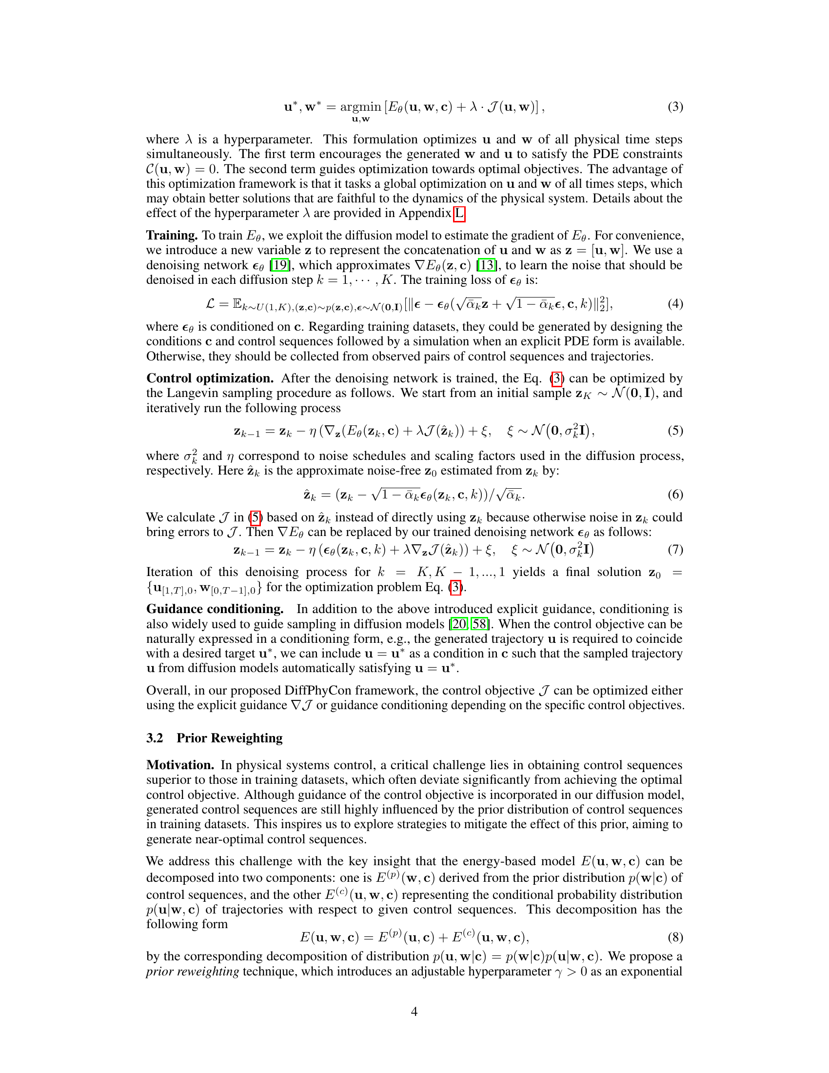
🔼 This figure illustrates the effect of prior reweighting on sampling from a joint distribution p(u,w). The top panel shows the cost function J(u,w). The middle panel shows the joint distribution p(w)p(u|w) when γ=1. The bottom panel shows the reweighted distribution pγ(w)p(u|w) when 0<γ<1. The reweighted distribution shifts the probability mass towards lower cost regions, improving the chances of sampling near-optimal solutions.
read the caption
Figure 2: Intuition of Prior Reweighting. The top surface illustrates the landscape of J(u, w), where the high-dimensional variables u and w are represented using one dimension. The middle and lower planes depict probability heatmaps for the reweighted distribution p^(w)p(u|w)/Z. Adjusting γ from γ = 1 (middle plane) to 0 < γ < 1 (lower plane), a better minimal of J (red dot in the lower plane) gains the chance to be sampled. This contrasts with the suboptimal red point in the middle plane highly influenced by the prior p(w).
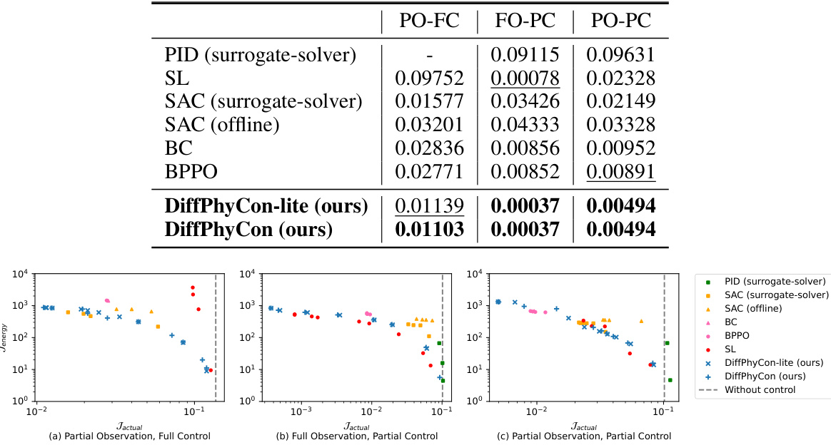
🔼 This figure compares the performance of various methods for controlling the 1D Burgers’ equation across three different experimental settings: partial observation, full control (PO-FC); full observation, partial control (FO-PC); and partial observation, partial control (PO-PC). Each setting presents a unique challenge related to the information available about the system state and the level of control exerted. The Pareto frontier illustrates the trade-off between minimizing the control energy (Jenergy) and minimizing the control error (Jactual). The figure shows that DiffPhyCon consistently achieves superior results, reaching lower Jactual values for a given Jenergy budget compared to other methods. This highlights its effectiveness in handling the complexities of partial observation and partial control scenarios.
read the caption
Figure 3: Pareto frontier of Jenergy VS. Jactual of different methods for 1D Burgers' equation.

🔼 This figure compares the generated control curves (opening angles of jellyfish wings over time) produced by different methods on three separate test jellyfish. The x-axis represents time, and the y-axis represents the opening angle. Each line represents a different method (DiffPhyCon-lite, DiffPhyCon, SAC (pseudo-online), SAC (offline), SL, MPC, BPPO, BC), with the resulting control objective J displayed for each jellyfish’s control sequence. This visualization helps to illustrate how different methods produce different control strategies for achieving the same goal (jellyfish movement). The figure shows DiffPhyCon’s ability to generate a smooth and effective control curve that leads to a better control objective compared to other methods.
read the caption
Figure 4: Comparison of generated control curves of three test jellyfish. The resulting control objective I for each curve is presented.

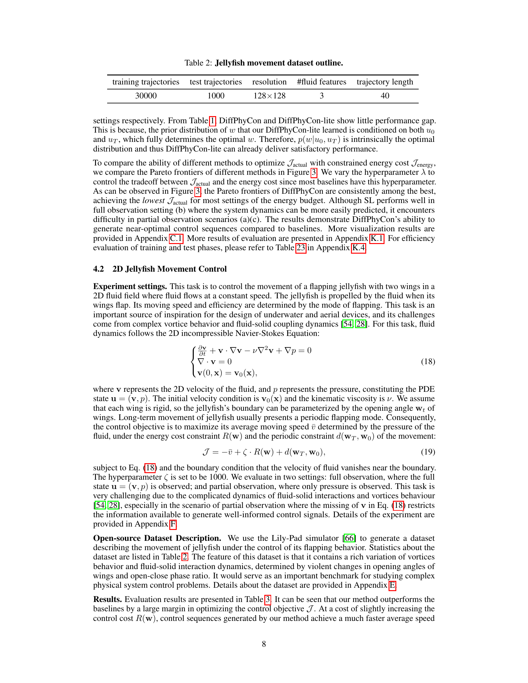
🔼 This figure visualizes the movement of a jellyfish and the surrounding fluid flow at different time points (t=0, 5, 10, 15, 20). The visualization is based on the results obtained using the DiffPhyCon method, specifically focusing on the control scenario illustrated in the middle subfigure of Figure 4. It showcases the dynamic interaction between the jellyfish’s movement (indicated by the brown shape) and the fluid flow (represented by the color map, where red indicates positive vorticity and blue indicates negative vorticity). The image provides a visual representation of how DiffPhyCon influences the jellyfish’s trajectory and the resulting fluid dynamics.
read the caption
Figure 5: Visualization of jellyfish movement and fluid field controlled by DiffPhyCon as in the middle subfigure of Figure 4.

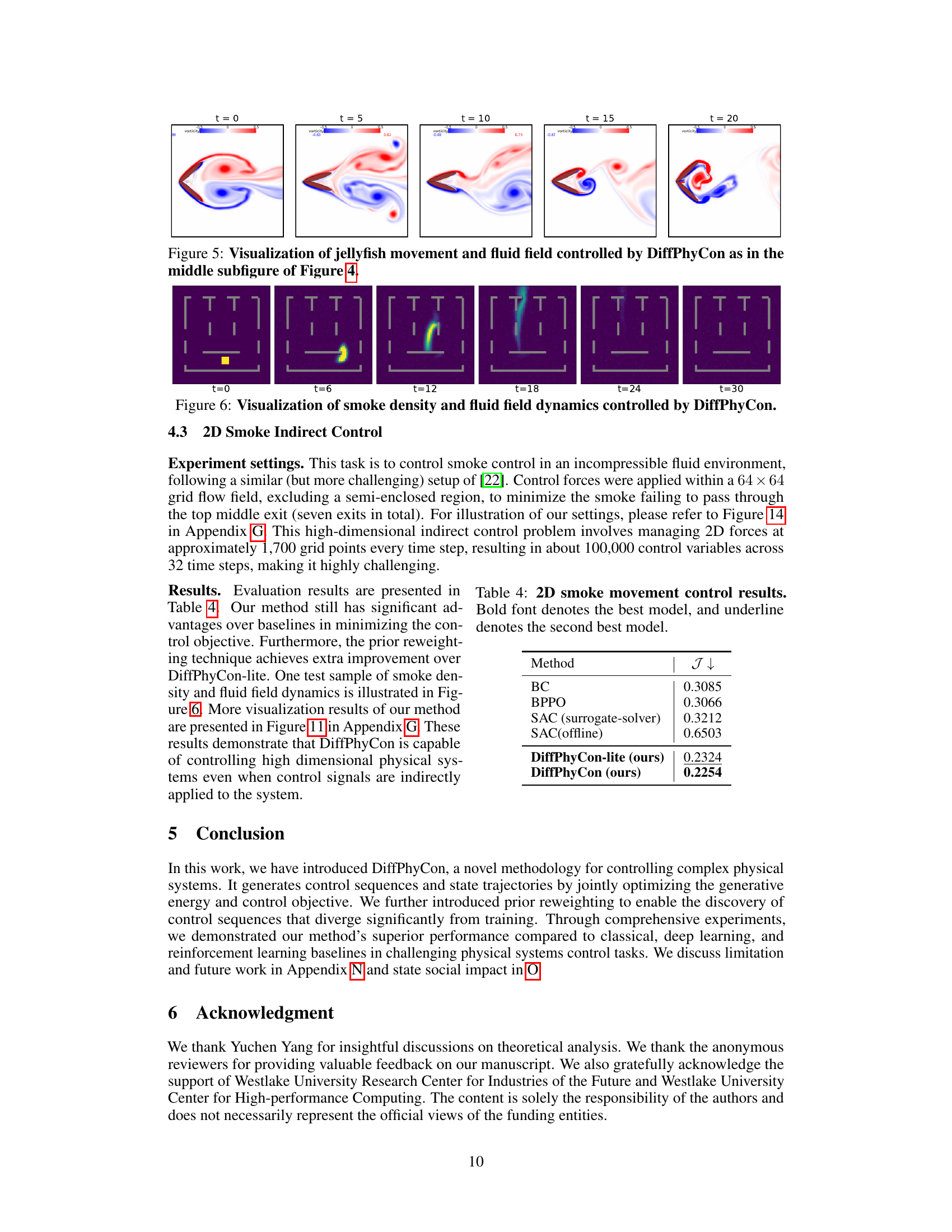
🔼 This figure visualizes the results of the 2D smoke indirect control task using the DiffPhyCon method. It shows a sequence of six snapshots (t=0, t=6, t=12, t=18, t=24, t=30) illustrating the evolution of smoke density and fluid field dynamics. The smoke, initially concentrated in a lower region, is guided by DiffPhyCon’s control signals to navigate through a complex channel with obstacles, ultimately aiming for a target exit at the top.
read the caption
Figure 6: Visualization of smoke density and fluid field dynamics controlled by DiffPhyCon.

🔼 This figure shows the results of applying various methods to control the 1D Burgers’ equation under the condition of full observation but partial control. It compares the performance of DiffPhyCon with baselines such as PID, SL, SAC, BC, and BPPO by visualizing the system state evolution over time for five randomly selected test samples. The plots illustrate how the different methods converge towards the target state, highlighting the effectiveness of DiffPhyCon in achieving a smooth and accurate convergence.
read the caption
Figure 7: Visualizations results of 1D Burgers' equation control under the FO-PC (full observation, partial control) setting. The curve for the system state ut of each time step t = 0,……, 10 under control is plotted for our method (DiffPhyCon) and baselines. The x-axis is the spatial coordinate and the y-axis is the value of the system state.

🔼 This figure shows a Pareto frontier, which is a curve illustrating the trade-off between two objectives: the energy cost (Jenergy) and the actual control error (Jactual). The Pareto frontier helps to visualize the performance of different methods for 1D Burgers’ equation control under various scenarios (partial observation, full control; full observation, partial control; partial observation, partial control). It allows for a comparison of different methods in their ability to achieve a balance between minimizing the control error while keeping the energy cost low. The different methods are compared in this trade-off.
read the caption
Figure 3: Pareto frontier of Jenergy VS. Jactual of different methods for 1D Burgers' equation.

🔼 This figure compares the performance of different methods in solving the 1D Burgers’ equation control problem under the full observation, partial control setting. The results are shown for five randomly selected samples from the test dataset. Each curve represents the evolution of the system state over time (t=0 to 10). The x-axis shows the spatial coordinate, and the y-axis shows the corresponding value of the system state. The figure visually demonstrates DiffPhyCon’s ability to effectively guide the system state towards the target state, compared to baseline methods like PID, SL, SAC, BC, and BPPO.
read the caption
Figure 7: Visualizations results of 1D Burgers' equation control under the FO-PC (full observation, partial control) setting. The curve for the system state ut of each time step t = 0,……, 10 under control is plotted for our method (DiffPhyCon) and baselines. The x-axis is the spatial coordinate and the y-axis is the value of the system state.

🔼 This figure shows more examples of 2D jellyfish simulations controlled by the DiffPhyCon method. Each row represents an example from the test dataset. Five snapshots of the simulation are shown for each example, showcasing the jellyfish’s movement and the corresponding fluid dynamics at different points in time (t = 0, 5, 10, 15, 20). The color schemes represent the vorticity of the fluid, highlighting the complex flow patterns generated by the jellyfish’s movements.
read the caption
Figure 10: More examples of 2D jellyfish simulation controlled by our method.

🔼 This figure visualizes the results of the 2D smoke control task using the DiffPhyCon method. It showcases three randomly selected test examples, each displayed as a row of six frames illustrating the progression of smoke density and the corresponding control force fields (horizontal and vertical) over time. The image highlights how the method guides the smoke towards the target exit.
read the caption
Figure 11: Examples of 2D smoke control results by our method. We present three randomly selected test examples. For each example, we show the generated smoke density map and control force fields in horizontal and vertical directions. Each row depicts six frames of movement. The smoke density in the first row corresponds to that in Figure 6.

🔼 This figure provides a high-level overview of the DiffPhyCon method, illustrating its three main stages: training, inference, and evaluation. The training phase involves learning two key distributions: the joint distribution of states and controls (orange), and the prior distribution of controls (blue). During inference, the model generates control sequences by minimizing a combined energy function, incorporating both learned distributions and guidance from the control objective. Finally, the generated control sequences are evaluated based on their performance in controlling the physical system.
read the caption
Figure 1: Overview of DiffPhyCon. The figure depicts the training (top), inference (bottom left), and evaluation (bottom right) of DiffPhyCon. Orange and blue colors respectively represent models learning the joint distribution pe(u, w) and the prior distribution pf(w). Through prior reweighting and guidance, DiffPhyCon is capable of generating superior control sequences.
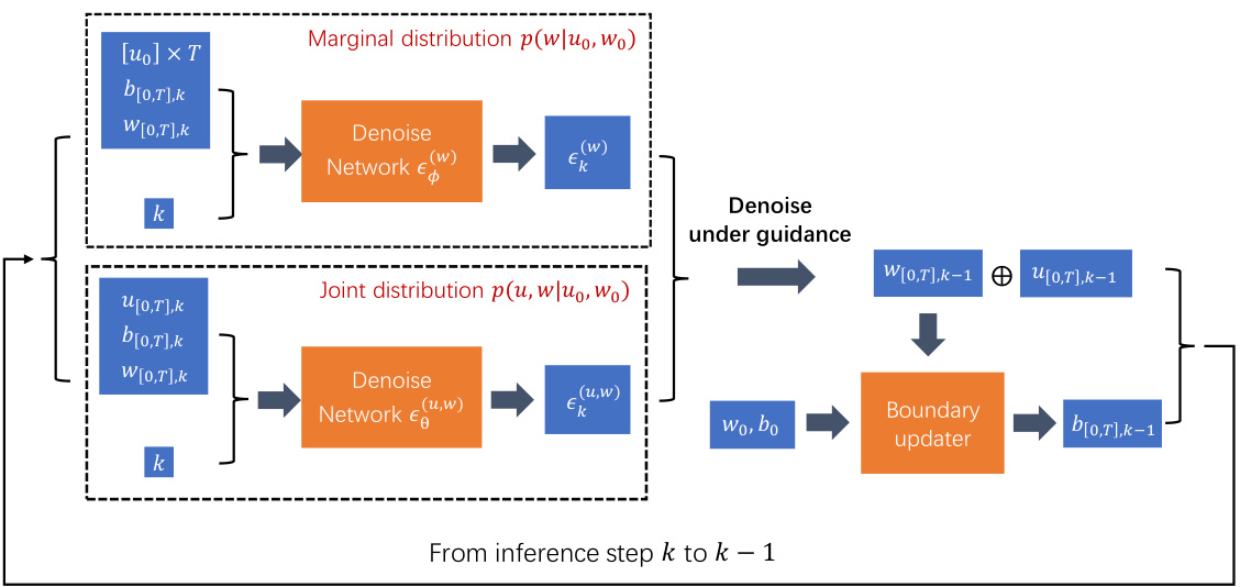
🔼 This figure shows a schematic overview of the DiffPhyCon method. The training phase involves learning the joint distribution of states and controls, as well as a prior distribution of control sequences. During inference, the model generates control sequences by denoising, incorporating prior reweighting and guidance to optimize for a specific objective. The evaluation step assesses the quality of the generated control sequences. The use of orange and blue colors helps distinguish the different models involved in the process.
read the caption
Figure 1: Overview of DiffPhyCon. The figure depicts the training (top), inference (bottom left), and evaluation (bottom right) of DiffPhyCon. Orange and blue colors respectively represent models learning the joint distribution pe(u, w) and the prior distribution pf(w). Through prior reweighting and guidance, DiffPhyCon is capable of generating superior control sequences.
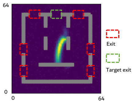
🔼 This figure shows the setup for a 2D smoke indirect control task. Panel (a) illustrates the overall layout of the environment, highlighting seven exits, obstacles, and the target exit (the top middle exit). Panel (b) emphasizes that control forces can only be applied to the peripheral regions, excluding the central semi-enclosed area where the smoke is initially placed. The goal is to minimize the smoke that doesn’t exit through the target exit.
read the caption
Figure 14: 2D smoke indirect control task. There are seven exits in total and the top middle one is the target exit (a). The control signals are only allowed to apply to peripheral regions (b). The control objective is to minimize the proportion of smoke failing to pass through the target exit.
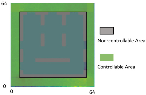
🔼 This figure shows the experimental setup for the 2D smoke indirect control task. Panel (a) illustrates the location of seven exits, with the central exit being the target. Panel (b) highlights the controllable region, which is limited to the perimeter of the simulation domain. The objective is to control airflow to maximize the amount of smoke exiting through the central target exit.
read the caption
Figure 14: 2D smoke indirect control task. There are seven exits in total and the top middle one is the target exit (a). The control signals are only allowed to apply to peripheral regions (b). The control objective is to minimize the proportion of smoke failing to pass through the target exit.

🔼 This figure shows the overall architecture of DiffPhyCon, a generative model for controlling complex physical systems. It illustrates the training process, where models learn the joint distribution of system trajectories and control sequences, as well as the prior distribution of control sequences. The inference process is also depicted, showing how DiffPhyCon utilizes prior reweighting and guidance to generate near-optimal control sequences that are faithful to the dynamics of the system. Finally, the evaluation process is shown, where the generated control sequences are evaluated based on predefined metrics.
read the caption
Figure 1: Overview of DiffPhyCon. The figure depicts the training (top), inference (bottom left), and evaluation (bottom right) of DiffPhyCon. Orange and blue colors respectively represent models learning the joint distribution pe(u, w) and the prior distribution pf(w). Through prior reweighting and guidance, DiffPhyCon is capable of generating superior control sequences.
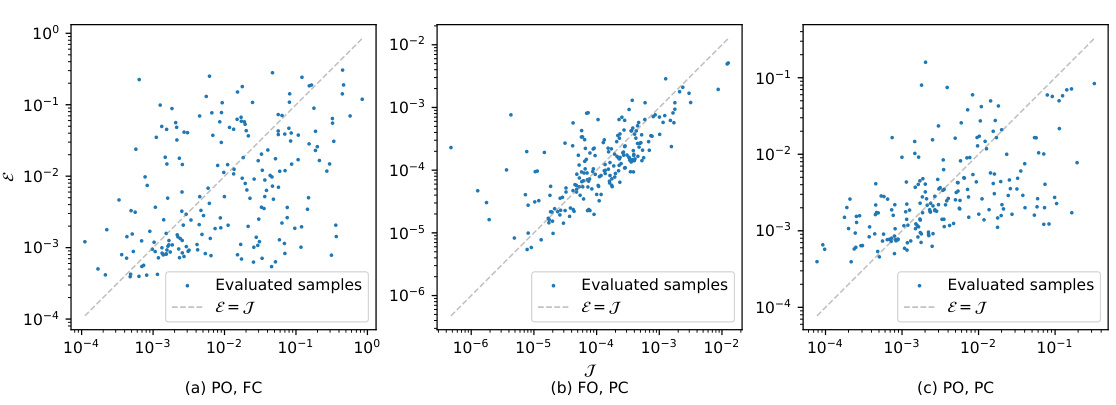
🔼 This figure compares the performance of different methods for controlling the 1D Burgers’ equation across three scenarios: partial observation with full control, full observation with partial control, and partial observation with partial control. The Pareto frontier plots the trade-off between the energy cost (Jenergy) and the actual control error (Jactual). DiffPhyCon consistently shows superior performance, achieving lower actual error for a given energy budget, particularly in scenarios with partial observations.
read the caption
Figure 3: Pareto frontier of Jenergy VS. Jactual of different methods for 1D Burgers' equation.
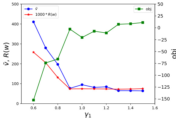
🔼 This figure visualizes the impact of the hyperparameter γ (prior reweighting intensity) on the performance of the DiffPhyCon model for the 2D jellyfish movement control task. The x-axis represents the hyperparameter γ₁, and the y-axis shows three different metrics: average speed (v̄), energy cost (1000*R(w)), and the control objective (obj). The plot reveals how adjusting γ₁ influences the model’s ability to balance the control objective with speed and energy constraints. The optimal γ₁ appears to be around 0.8 - 1.0, resulting in a fast average speed and relatively lower energy consumption while achieving a good control objective. Values outside this range show a significant decrease in average speed, while values less than 0.6 show the model is overly constrained by the prior distribution, resulting in suboptimal performance. The plot shows a Pareto frontier-type relationship between these three objectives.
read the caption
Figure 17: Results of different γ in DiffPhyCon on 2D jellyfish movement control task.
🔼 This figure illustrates the overall workflow of the DiffPhyCon model. The training phase involves learning a joint probability distribution over system trajectories (u) and control sequences (w), as well as a prior distribution of control sequences. The inference phase utilizes this learned distribution, along with prior reweighting and guidance, to generate near-optimal control sequences. Finally, the evaluation phase assesses the quality of the generated sequences.
read the caption
Figure 1: Overview of DiffPhyCon. The figure depicts the training (top), inference (bottom left), and evaluation (bottom right) of DiffPhyCon. Orange and blue colors respectively represent models learning the joint distribution pe(u, w) and the prior distribution pf(w). Through prior reweighting and guidance, DiffPhyCon is capable of generating superior control sequences.

🔼 This figure shows a schematic overview of the DiffPhyCon method. It illustrates the training phase, where models learn the joint distribution of states and controls and the prior distribution of controls. The inference phase uses the learned models with prior reweighting to generate optimal control sequences. Finally, the evaluation phase assesses the quality of generated control sequences.
read the caption
Figure 1: Overview of DiffPhyCon. The figure depicts the training (top), inference (bottom left), and evaluation (bottom right) of DiffPhyCon. Orange and blue colors respectively represent models learning the joint distribution pe(u, w) and the prior distribution pf(w). Through prior reweighting and guidance, DiffPhyCon is capable of generating superior control sequences.
More on tables
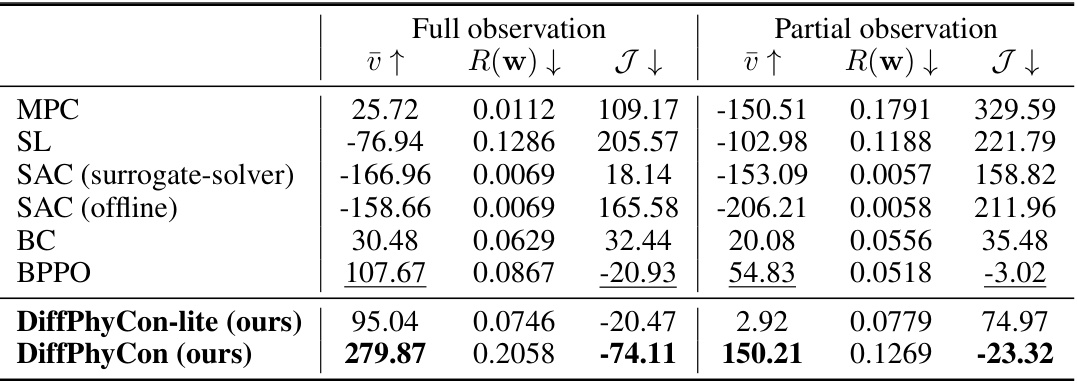
🔼 This table presents the results of applying different methods to the 2D jellyfish movement control task. The table is split into two sections: ‘Full observation’ and ‘Partial observation’, representing different levels of observability. Each method is evaluated across three metrics: the average speed (ū ↑), the energy cost (R(w) ↓), and the control objective (J ↓). Bold values indicate the best performing method for each metric in each setting, and underlined values indicate the second-best performance. This comparison highlights the relative effectiveness of DiffPhyCon in achieving near-optimal performance compared to various baseline methods, particularly in scenarios with reduced observability.
read the caption
Table 3: 2D jellyfish movement control results. Bold font denotes the best model, and underline denotes the second best model.
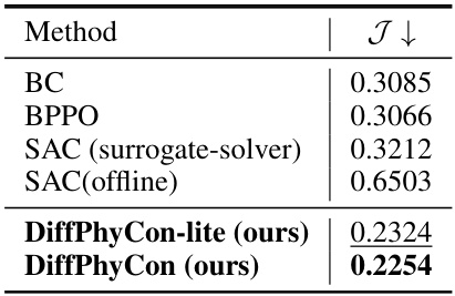
🔼 This table presents the results of 2D smoke movement control experiments, comparing the performance of different methods, namely BC, BPPO, SAC (with both surrogate-solver and offline versions), and the proposed DiffPhyCon (with both DiffPhyCon-lite and DiffPhyCon versions). The table shows the control objective (J↓) achieved by each method. The best performing method (lowest J value) is indicated in bold, and the second-best performing method is underlined. The results highlight the superior performance of the DiffPhyCon methods compared to the baseline methods.
read the caption
Table 4: 2D smoke movement control results. Bold font denotes the best model, and underline denotes the second best model.
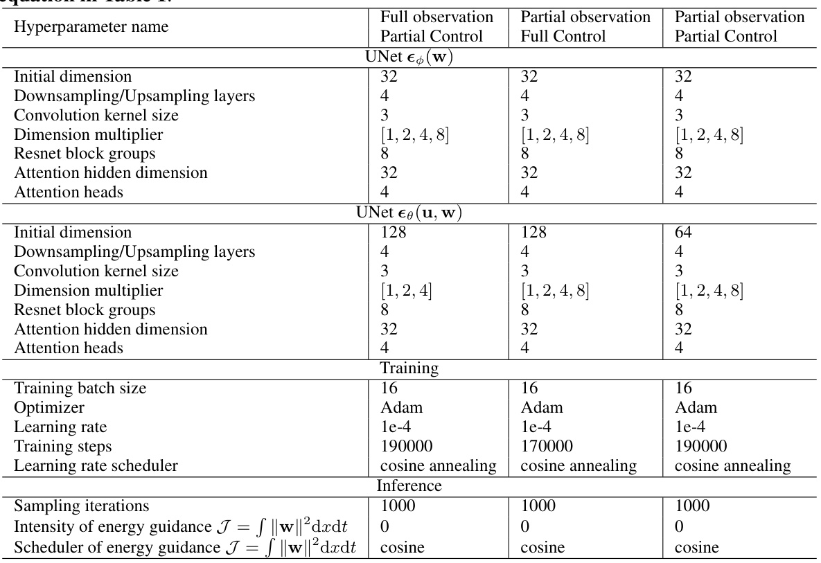
🔼 This table lists the hyperparameters used for training the UNet models in the 1D Burgers’ equation control experiments. It details the network architecture and training parameters for three different experimental settings: full observation partial control, partial observation full control, and partial observation partial control. The hyperparameters include initial dimension, number of downsampling/upsampling layers, convolution kernel size, dimension multiplier, number of ResNet block groups, attention hidden dimension, and number of attention heads. Training hyperparameters such as batch size, optimizer, learning rate, number of training steps, and learning rate scheduler are also specified. Finally, inference-related hyperparameters like sampling iterations and the intensity/scheduler of energy guidance are included.
read the caption
Table 5: Hyperparameters of the UNet architecture and training for the results of 1D Burgers' equation in Table 1.
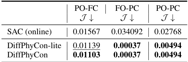
🔼 This table presents a comparison of the best achieved Jactual (actual control error) across different methods for controlling the 1D Burgers’ equation. The results are separated into three settings representing different observation and control scenarios. The best performing model in each setting is highlighted in bold, and the second-best model is underlined. The table provides a quantitative comparison of the effectiveness of various methods for physical system control, highlighting the superior performance of the DiffPhyCon method.
read the caption
Table 1: Best Jactual achieved in 1D Burgers's equation control. Bold font denotes the best model, and underline denotes the second best model.

🔼 This table presents the best achieved values for the actual control error (Jactual) across different control methods for the 1D Burgers’ equation. The results are categorized by three experimental settings: Partial Observation, Full Control (PO-FC); Full Observation, Partial Control (FO-PC); and Partial Observation, Partial Control (PO-PC). The lowest values of Jactual represent the most effective control, indicating the best model performance in minimizing the error between the achieved and target state of the system under the constraints of each setting.
read the caption
Table 1: Best Jactual achieved in 1D Burgers's equation control. Bold font denotes the best model, and underline denotes the second best model.

🔼 This table presents the best and second-best values for the actual control error (Jactual) achieved by various methods in a 1D Burgers’ equation control task. The methods are compared across three experimental settings: partial observation, full control (PO-FC); full observation, partial control (FO-PC); and partial observation, partial control (PO-PC). The bold values indicate the best-performing method for each setting, while the underlined values represent the second-best.
read the caption
Table 1: Best Jactual achieved in 1D Burgers's equation control. Bold font denotes the best model, and underline denotes the second best model.
🔼 This table presents the best and second-best Jactual values achieved by different methods in controlling the 1D Burgers’ equation under three different settings (PO-FC, FO-PC, and PO-PC). The lower the Jactual value, the better the control performance. The table highlights DiffPhyCon’s superior performance compared to other methods, including traditional methods (PID), supervised learning (SL), and reinforcement learning techniques (SAC, BC, BPPO).
read the caption
Table 1: Best Jactual achieved in 1D Burgers's equation control. Bold font denotes the best model, and underline denotes the second best model.

🔼 This table presents the best achieved Jactual values (the control error) for different methods in the 1D Burgers’ equation control task. It compares the performance of DiffPhyCon and various baselines (PID, supervised learning (SL), reinforcement learning methods SAC, BC, and BPPO) under three different experimental settings: partial observation and full control (PO-FC), full observation and partial control (FO-PC), and partial observation and partial control (PO-PC). Bold font highlights the best-performing model for each setting, while underlined values indicate the second-best.
read the caption
Table 1: Best Jactual achieved in 1D Burgers's equation control. Bold font denotes the best model, and underline denotes the second best model.
🔼 This table presents the best and second-best Jactual (actual control error) achieved by different methods in the 1D Burgers’ equation control task. The methods compared include traditional control methods (PID), supervised learning (SL), reinforcement learning (RL) methods (SAC, BC, BPPO), and the proposed DiffPhyCon and DiffPhyCon-lite. The results are categorized by three experimental settings: partial observation, full control (PO-FC); full observation, partial control (FO-PC); and partial observation, partial control (PO-PC). Bold font indicates the best-performing method for each setting, while underlined text indicates the second-best.
read the caption
Table 1: Best Jactual achieved in 1D Burgers's equation control. Bold font denotes the best model, and underline denotes the second best model.
🔼 This table presents the best Jactual values achieved by different methods in controlling the 1D Burgers’ equation under three different experimental settings: partial observation, full control (PO-FC); full observation, partial control (FO-PC); and partial observation, partial control (PO-PC). The results show DiffPhyCon achieving the best performance across all three settings, highlighting its superior performance compared to classical methods (PID), supervised learning (SL), and reinforcement learning methods (SAC, BC, BPPO).
read the caption
Table 1: Best Jactual achieved in 1D Burgers's equation control. Bold font denotes the best model, and underline denotes the second best model.
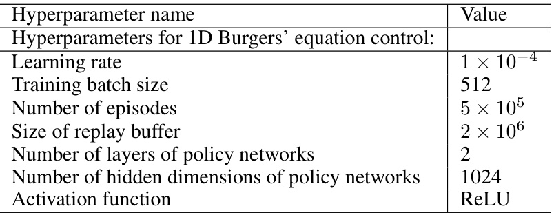
🔼 This table presents the best values of the actual control error (Jactual) achieved by different methods in the 1D Burgers’ equation control task. The methods compared include traditional methods (PID), supervised learning (SL), reinforcement learning (RL) methods (SAC, BC, BPPO), and the proposed DiffPhyCon method (with and without prior reweighting). Bold font indicates the best performing model overall, and underlined values denote the second-best model for each control setting. This allows for a direct comparison of the performance of different control algorithms for this specific task, highlighting the strengths of DiffPhyCon.
read the caption
Table 1: Best Jactual achieved in 1D Burgers's equation control. Bold font denotes the best model, and underline denotes the second best model.
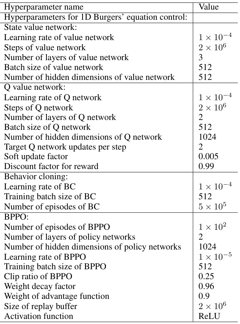
🔼 This table presents the best Jactual (actual control error) achieved by different methods for the 1D Burgers’ equation control task. The results are categorized by three experimental settings: Partial Observation, Full Control (PO-FC); Full Observation, Partial Control (FO-PC); and Partial Observation, Partial Control (PO-PC). The best performing method for each setting is indicated in bold font, while the second best is underlined. The table highlights the relative performance of DiffPhyCon compared to several baselines, including PID, Supervised Learning (SL), Soft Actor-Critic (SAC), Behavior Cloning (BC), and Behavior Proximal Policy Optimization (BPPO).
read the caption
Table 1: Best Jactual achieved in 1D Burgers's equation control. Bold font denotes the best model, and underline denotes the second best model.
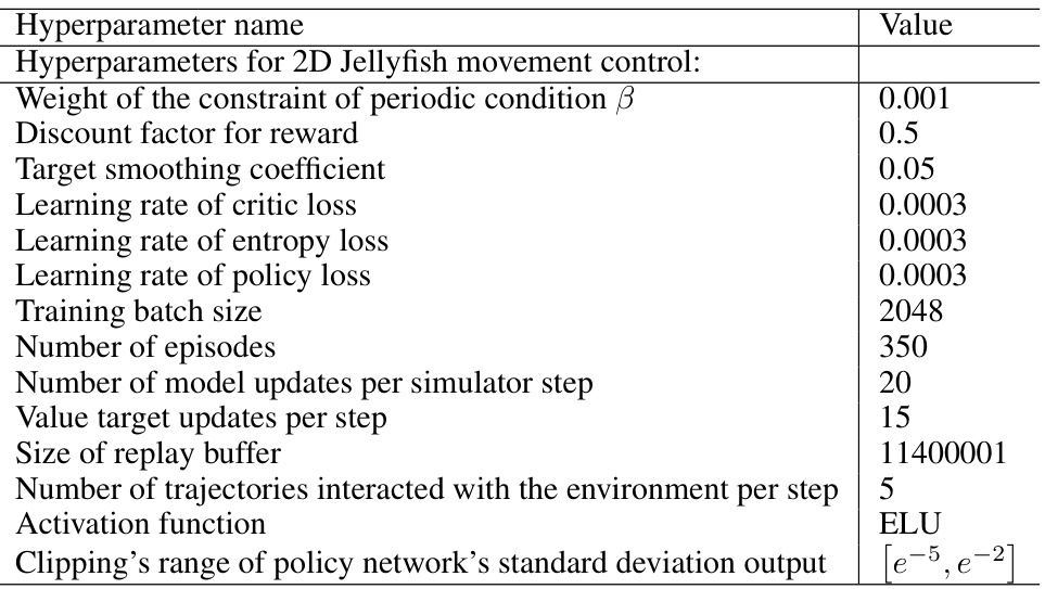
🔼 This table presents the results of 2D jellyfish movement control experiments, comparing the performance of different methods across two settings: full observation and partial observation. The best performing model is highlighted in bold, and the second best is underlined. The table displays the average speed, energy consumption, and overall performance metric for each method. This provides a quantitative comparison of DiffPhyCon and its baselines in a complex control task.
read the caption
Table 3: 2D jellyfish movement control results. Bold font denotes the best model, and underline denotes the second best model.

🔼 This table presents the best values achieved for the ‘Jactual’ metric in a 1D Burgers’ equation control experiment, comparing different methods. The Jactual metric represents the control error. Bold typeface indicates the best performing model overall, while underlined text highlights the second-best model. The table allows for a quick comparison of the effectiveness of various control approaches in minimizing the control error.
read the caption
Table 1: Best Jactual achieved in 1D Burgers's equation control. Bold font denotes the best model, and underline denotes the second best model.
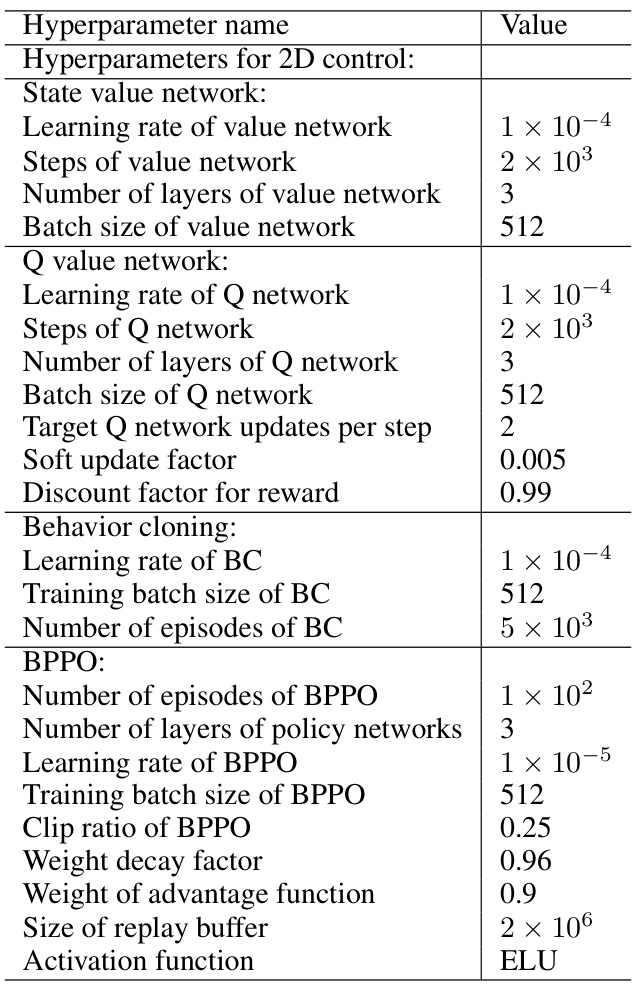
🔼 This table presents a comparison of different control methods on a 2D jellyfish movement control task. The results are separated into ‘Full observation’ and ‘Partial observation’ settings, reflecting the amount of information available to the controller. For each method, it shows the average speed, the energy cost, and the control objective values. The best performing model in each category is bolded, and the second-best model is underlined.
read the caption
Table 3: 2D jellyfish movement control results. Bold font denotes the best model, and underline denotes the second best model.

🔼 This table presents the best and second-best Jactual values achieved by different methods in the 1D Burgers’ equation control task, categorized by the experimental setting (PO-FC, FO-PC, PO-PC). Jactual represents the actual control error, a key metric in evaluating the performance of different control methods. The best-performing method in each setting is highlighted in bold font, while the second-best method is underlined.
read the caption
Table 1: Best Jactual achieved in 1D Burgers's equation control. Bold font denotes the best model, and underline denotes the second best model.
🔼 This table presents the best achieved Jactual (actual control error) for different methods in the 1D Burgers’ equation control task. The results are categorized by three experimental settings: PO-FC (Partial Observation, Full Control), FO-PC (Full Observation, Partial Control), and PO-PC (Partial Observation, Partial Control). The lowest Jactual values indicate the most effective control methods for each setting. Bold text highlights the best-performing model in each setting, while underlined text indicates the second-best model.
read the caption
Table 1: Best Jactual achieved in 1D Burgers's equation control. Bold font denotes the best model, and underline denotes the second best model.

🔼 This table presents the results of the 2D jellyfish movement control experiment. It compares the performance of different methods (MPC, SL, SAC (offline), SAC (surrogate-solver), BC, BPPO, DiffPhyCon-lite, and DiffPhyCon) in both full observation and partial observation settings. The metrics reported include the control objective (J), the energy cost (R(w)), and the average speed (ū). Bold values indicate the best performing model for each metric and setting, while underlined values show the second-best results.
read the caption
Table 3: 2D jellyfish movement control results. Bold font denotes the best model, and underline denotes the second best model.

🔼 This table presents the results of applying different control methods to a 2D jellyfish movement control task. The results are split into two settings: ‘Full observation’ and ‘Partial observation’. For each method and setting, the table shows the average speed (ū↑), energy cost (R(w)↓), control objective (I↓), and the energy-speed tradeoff. Bold font indicates the best-performing method in each column, while underlined values represent the second-best method. The table demonstrates the relative performance of various methods under different conditions of observability.
read the caption
Table 3: 2D jellyfish movement control results. Bold font denotes the best model, and underline denotes the second best model.

🔼 This table compares the performance of SAC and DiffPhyCon in controlling jellyfish movement, highlighting the impact of myopic failure modes in SAC. The table presents results for average speed, energy cost (R(w)), the overall control objective (I), and periodicity error, showing that DiffPhyCon significantly outperforms SAC, particularly in achieving a much higher average speed while maintaining a low periodicity error.
read the caption
Table 22: Results of myopic failure modes of SAC on 2D jellyfish movement control.

🔼 This table presents the best and second-best Jactual (actual control error) values achieved by different methods in controlling the 1D Burgers’ equation. The results are categorized across three experimental settings: PO-FC (Partial Observation - Full Control), FO-PC (Full Observation - Partial Control), and PO-PC (Partial Observation - Partial Control). The bold font highlights the best-performing method for each setting, while underlined values indicate the second-best performance. This comparison demonstrates DiffPhyCon’s superior performance in minimizing the control error compared to established methods.
read the caption
Table 1: Best Jactual achieved in 1D Burgers's equation control. Bold font denotes the best model, and underline denotes the second best model.

🔼 This table compares the training and inference time for different methods used in the 2D jellyfish movement control task. It shows that DiffPhyCon and DiffPhyCon with DDIM (a faster sampling method) have similar training times but DiffPhyCon has a significantly longer inference time than other methods. The training times are reported along with the hardware used, and the inference time is standardized to a Tesla-V100 GPU with 8 CPUs for comparison.
read the caption
Table 24: Efficiency comparison on 2D jellyfish movement. Inference time is tested on a Tesla-V100 GPU with 8 CPUs.

🔼 This table presents the results of applying DiffPhyCon with different values of the hyperparameter γ on the FO-PC (Full Observation, Partial Control) setting of the 1D Burgers equation control task. It shows the impact of γ on both the actual control error (Jactual) and the mean squared error between the generated states and the ground truth states (State MSE). The results demonstrate the relative insensitivity of performance to changes in γ in this particular experimental setting.
read the caption
Table 25: Results of different γ in DiffPhyCon on FO-PC 1D Burgers equation control task.

🔼 This table presents the best and second-best Jactual (actual control error) achieved by different methods for the 1D Burgers’ equation control task. The methods include PID, SL (supervised learning), SAC (soft actor-critic) with offline and surrogate-solver versions, BC (behaviour cloning), BPPO (behaviour proximal policy optimization), DiffPhyCon-lite, and DiffPhyCon. The results are broken down by three experimental settings: PO-FC (partial observation, full control), FO-PC (full observation, partial control), and PO-PC (partial observation, partial control). The bold values indicate the best performance within each setting, while underlined values show the second-best performance.
read the caption
Table 1: Best Jactual achieved in 1D Burgers's equation control. Bold font denotes the best model, and underline denotes the second best model.

🔼 This table presents the results of the DiffPhyCon model’s performance on the 1D Burgers’ equation control task with partial observation and partial control (PO-PC). It shows the impact of the hyperparameter γ (prior reweighting intensity) on the control error (Jactual) and state mean squared error (State MSE). Different values of γ were tested to evaluate its influence on the model’s ability to find near-optimal control sequences.
read the caption
Table 27: Results of different γ in DiffPhyCon on PO-PC 1D Burgers equation control task.

🔼 This table presents the results of the 2D jellyfish movement control experiments. It compares the performance of different methods (MPC, SL, SAC, BC, BPPO, DiffPhyCon-lite, and DiffPhyCon) in two settings: full observation and partial observation. The metrics used to evaluate performance are the average speed (ū), the energy cost (R(w)), the objective function (J), and the periodicity error. Bold font indicates the best-performing method in each metric, while underlined text highlights the second-best performing method.
read the caption
Table 3: 2D jellyfish movement control results. Bold font denotes the best model, and underline denotes the second best model.

🔼 This table presents the best Jactual (actual control error) achieved by different methods in the 1D Burgers’ equation control task. The results are broken down by three experimental settings: partial observation, full control (PO-FC); full observation, partial control (FO-PC); and partial observation, partial control (PO-PC). The best performing model for each setting is shown in bold font, while the second-best is underlined. The table highlights the superior performance of DiffPhyCon compared to other methods.
read the caption
Table 1: Best Jactual achieved in 1D Burgers's equation control. Bold font denotes the best model, and underline denotes the second best model.

🔼 This table presents the best Jactual (actual control error) achieved by different methods in a 1D Burgers’ equation control task. The results are compared across three experimental settings: partial observation, full control (PO-FC); full observation, partial control (FO-PC); and partial observation, partial control (PO-PC). The best performing model in each setting is indicated in bold font, and the second-best model is underlined. The table shows the quantitative performance comparison of DiffPhyCon against various classical, supervised learning, and reinforcement learning baselines.
read the caption
Table 1: Best Jactual achieved in 1D Burgers's equation control. Bold font denotes the best model, and underline denotes the second best model.

🔼 This table presents the results of applying DiffPhyCon with varying lambda (λ) values on the PO-FC (Partial Observation, Full Control) setting for the 1D Burgers’ equation control task. It shows the impact of λ on the actual objective function (Jactual), the mean squared error of the system state (State MSE), and the energy cost (Jenergy) for different λ values. The results help to understand the tradeoff between control accuracy and energy consumption.
read the caption
Table 31: Results of different λ for Jenergy of DiffPhyCon in PO-FC 1D Burgers equation control task.

🔼 This table shows the impact of the hyperparameter λ on the energy cost (Jenergy) and control error (Jactual) of the DiffPhyCon model in the full observation, partial control setting of the 1D Burgers’ equation control task. Different values of λ represent different balances between minimizing the control error and minimizing energy consumption. The State MSE column shows the mean squared error between the generated system state and the ground truth state. The results show how the balance shifts as λ varies.
read the caption
Table 30: Results of different λ for Jenergy of DiffPhyCon in FO-PC 1D Burgers equation control task.
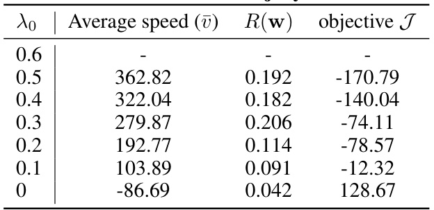
🔼 This table presents the results of the 2D jellyfish movement control experiments using DiffPhyCon with varying λ₀ values. The columns show the average speed (ū), energy cost (R(w)), and the control objective (J) for different hyperparameter settings. It demonstrates how the control objective changes in relation to the control strategy hyperparameter.
read the caption
Table 33: Results of different λ₀ in DiffPhyCon on 2D jellyfish movement control task.

🔼 This table lists the hyperparameters used for both the network architecture and training process in the 2D experiment of the paper. It shows the settings used for the full observation and partial observation scenarios, indicating the batch size, optimizer, learning rate, and loss function used for each. These hyperparameters are crucial for reproducibility of the experimental results.
read the caption
Table 7: Hyperparameters of network architecture and training for the 2D experiment.

🔼 This table presents the results of the DiffPhyCon-lite model on a more challenging jellyfish control task, where the jellyfish’s boundaries are soft and flexible. It shows the average speed achieved, the energy cost (R(w)), and the overall control objective (J) obtained by the model on this task. This table demonstrates the scalability and robustness of the DiffPhyCon-lite method in handling complex, high-dimensional control problems.
read the caption
Table 35: Performance of DiffPhyCon-lite on the finer-grained jellyfish boundary control task.
Full paper#

