TL;DR#
Meta-learning, enabling models to learn from limited examples, is gaining traction. However, current methods often lack robustness to variations in task distributions, particularly concerning “tail tasks” – those with unpredictable behavior. This research focuses on improving robustness by minimizing the risk associated with these tail tasks. The existing two-stage approach is computationally inefficient and lacks theoretical grounding.
The researchers recast the two-stage method as a max-min optimization problem, leveraging the Stackelberg game concept. This provides a solution concept, establishes a convergence rate, and derives a generalization bound, connecting the method to quantile estimation. They further replace the Monte Carlo method with kernel density estimation for practical improvement. Extensive evaluations demonstrate the effectiveness of their enhanced approach, showcasing its scalability and improved robustness across various benchmarks.
Key Takeaways#
Why does it matter?#
This paper is crucial because it tackles the critical issue of robustness in meta-learning, particularly relevant to the growing use of large language models in risk-sensitive applications. By providing theoretical justifications and practical enhancements to tail-risk minimization, it advances the field and opens avenues for creating more reliable and adaptable AI systems.
Visual Insights#
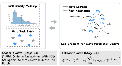
🔼 This figure illustrates the two-stage optimization process in distributionally robust meta-learning, framed as a Stackelberg game. Stage I (the leader’s move) involves modeling the risk distribution using kernel density estimation (KDE) and selecting a subset of tasks based on their risk. Stage II (the follower’s move) updates the meta-learner’s parameters using a sub-gradient method based on the screened subset from Stage I. The figure highlights the interplay between risk assessment and parameter updates, demonstrating how this approach increases robustness in meta-learning.
read the caption
Figure 1: Illustration of optimization stages in distributionally robust meta learning from a Stackelberg game. Given the DR-MAML example, the pipeline can be interpreted as bi-level optimization: the leader's move for characterizing tail task risk and the follower's move for robust fast adaptation.

🔼 This table presents the average 5-way 1-shot classification accuracies achieved by different meta-learning methods on the mini-ImageNet dataset. The results are averaged over three runs, and the standard deviations are also reported. The best-performing method for each metric (average, worst-case, and CVaR) is highlighted in bold. The confidence level (α) used for the CVaR calculation is 0.5.
read the caption
Table 1: Average 5-way 1-shot classification accuracies in mini-ImageNet with reported standard deviations (3 runs). With α = 0.5, the best results are in bold.
In-depth insights#
Tail Risk in Meta-Learning#
Tail risk, the probability of extreme negative events, presents a significant challenge in meta-learning, where the goal is to learn quickly from few examples. Traditional meta-learning methods often focus on average performance, neglecting the potential for catastrophic failures on rare, unseen tasks. This is problematic for real-world applications, especially in high-stakes domains like healthcare or finance. Addressing tail risk requires new methods that move beyond average performance metrics and incorporate robustness considerations. Distributionally robust optimization techniques, which account for worst-case scenarios, show promise in improving robustness. However, these methods can be computationally expensive. Quantile estimation techniques offer a practical way to identify and mitigate tail risk. By focusing on the upper quantiles of the performance distribution, these techniques aim to minimize the impact of extreme events while maintaining reasonable average performance. Future research in this area will likely focus on developing more efficient algorithms for quantile estimation and integrating them seamlessly into meta-learning frameworks. Additionally, exploring different risk measures and incorporating domain-specific knowledge are crucial to tailor solutions to specific applications.
Stackelberg Equilibrium#
The concept of Stackelberg Equilibrium, within the context of a research paper focusing on robust meta-learning, offers a powerful framework for analyzing a two-stage optimization strategy. Modeling the interaction between task selection (the leader) and model parameter updates (the follower) as a game, this approach provides a structured way to understand the dynamics of the learning process. The equilibrium point represents a robust solution, where the leader’s choice of tasks anticipates and optimizes for the follower’s best response, leading to improved adaptation robustness in the face of distributional shifts. The theoretical analysis of the Stackelberg game allows for establishing convergence rates, generalization bounds, and the exploration of asymptotic behavior, providing a more nuanced view than traditional risk minimization approaches. While the equilibrium concept itself can be computationally challenging to achieve, approximating it through methods like the two-stage strategy provides a practical balance between theoretical rigor and real-world applicability.
KDE Quantile Estimation#
Kernel Density Estimation (KDE) offers a powerful, non-parametric approach to quantile estimation, particularly valuable when dealing with complex or unknown data distributions. Unlike traditional methods that assume specific distributions, KDE constructs a smooth probability density function by weighting nearby data points, allowing for flexible representation of the underlying distribution’s shape. This flexibility is crucial when the true distribution is uncertain or non-standard, a common situation in meta-learning contexts. The smooth density function generated by KDE allows for accurate interpolation, leading to a more precise calculation of quantiles compared to methods like the crude Monte Carlo, which can be prone to significant approximation errors. However, KDE’s computational cost can be relatively high, particularly with large datasets. Bandwidth selection is also a critical factor, influencing the smoothness and accuracy of the resulting density and consequently the estimated quantiles. Careful consideration of these computational aspects and the selection of appropriate bandwidth parameters are essential for effective implementation of KDE in quantile estimation.
Asymptotic Convergence#
Asymptotic convergence, in the context of machine learning, particularly meta-learning, refers to the behavior of an algorithm’s performance as the number of iterations approaches infinity. It’s a crucial concept for understanding the long-term stability and effectiveness of the learning process. In meta-learning, where models learn to learn from a distribution of tasks, asymptotic convergence ensures that the model’s parameters converge to a stable state, even when presented with previously unseen tasks. However, this convergence isn’t necessarily to a global optimum; local optima or saddle points are possible, especially with non-convex optimization problems commonly encountered in deep learning. The speed of convergence, often expressed as a convergence rate, is also critical: a fast convergence rate is preferable since it means the algorithm reaches a satisfactory level of performance with fewer computations. The theoretical analysis of asymptotic convergence commonly involves establishing bounds on the error, which can provide guarantees on the model’s generalization performance. Establishing these bounds often requires assumptions on the task distribution, the model architecture, and the optimization algorithm used. Therefore, a complete understanding of asymptotic convergence necessitates a multifaceted approach that takes into account theoretical analysis, algorithmic design, and empirical evaluation.
Large Model Scalability#
Scaling large language models (LLMs) presents significant challenges. Computational cost explodes with model size, demanding extensive hardware and energy resources. Memory limitations restrict batch size and sequence length during training, impacting optimization and generalization. Deployment complexities arise from the need for specialized infrastructure and efficient inference methods. Data requirements also increase substantially, requiring massive datasets for effective training and fine-tuning. Addressing these challenges requires innovations in model architecture, training techniques (e.g., efficient training algorithms, model parallelism), and hardware acceleration to improve both training and inference speeds and reduce the overall resource footprint of LLMs. Research into efficient model compression and quantization is crucial for deploying large models on resource-constrained devices. Successfully scaling LLMs requires a multi-faceted approach encompassing architectural, algorithmic, and infrastructural improvements.
More visual insights#
More on figures

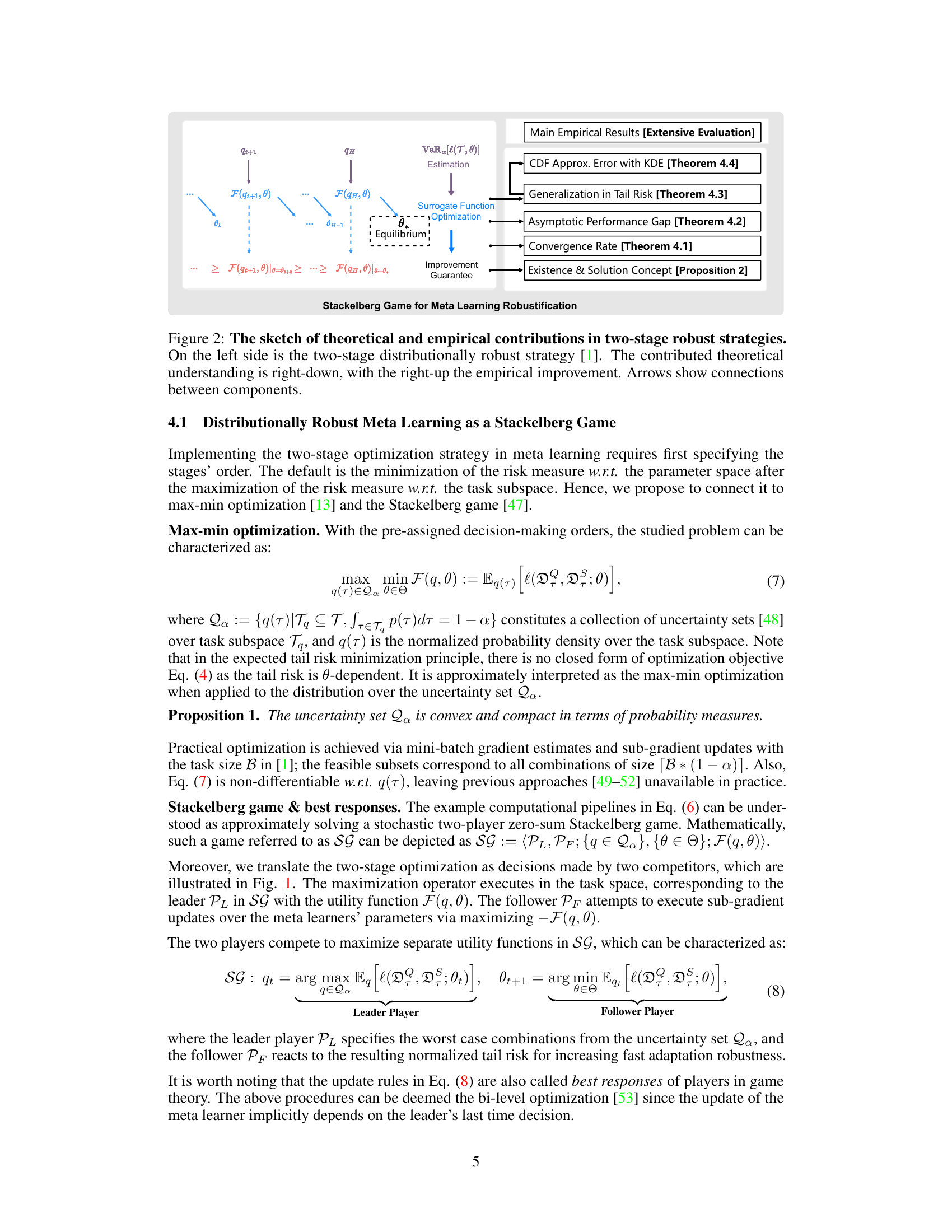
🔼 This figure summarizes the theoretical and empirical contributions of the paper’s proposed two-stage robust strategy. The left side depicts the original two-stage strategy from existing work [1]. The right-hand side shows the contributions made by this paper. The theoretical contributions, including the solution concept, convergence rate analysis, and generalization bound, are shown in the lower right. The empirical improvements, which involve extensive evaluations, are shown in the upper right. The arrows illustrate the relationships and connections between different parts of the approach and the findings.
read the caption
Figure 2: The sketch of theoretical and empirical contributions in two-stage robust strategies. On the left side is the two-stage distributionally robust strategy [1]. The contributed theoretical understanding is right-down, with the right-up the empirical improvement. Arrows show connections between components.

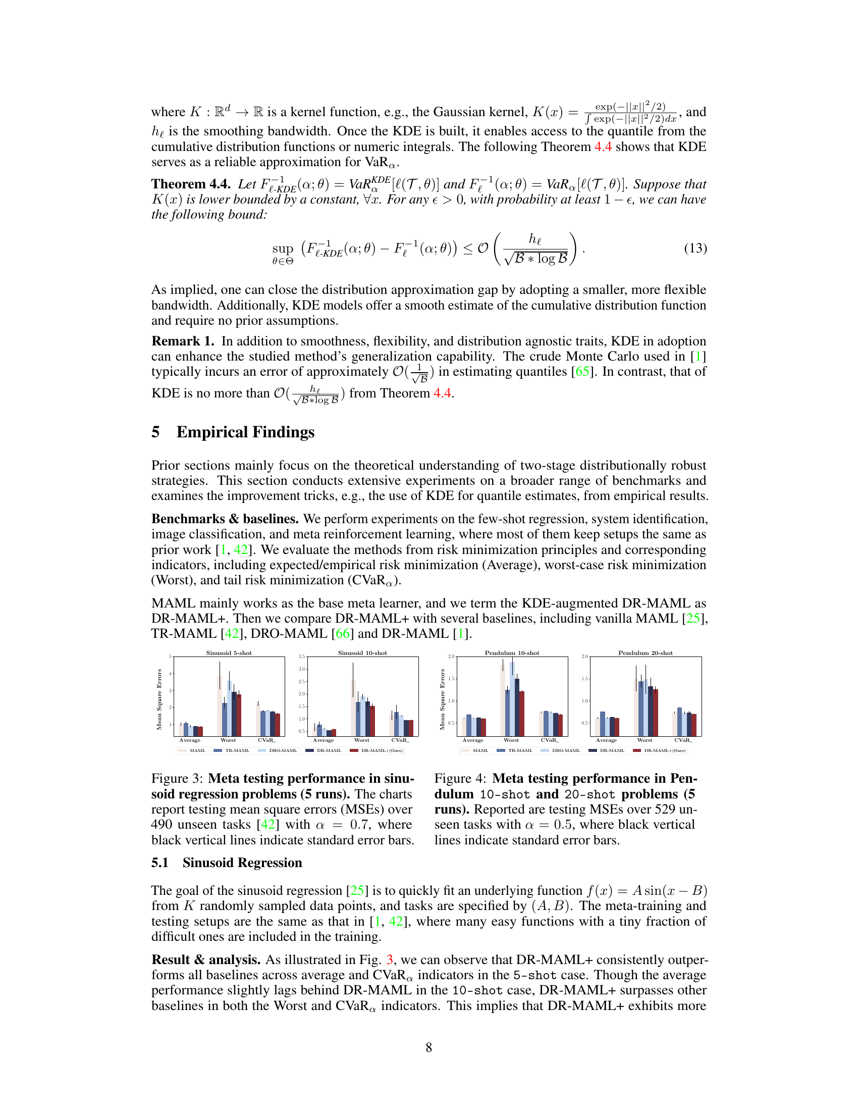
🔼 This figure presents the results of meta-testing on sinusoid regression problems. Five runs were conducted, and the mean squared error (MSE) is reported for each of the algorithms being compared. The x-axis shows the type of risk being minimized (Average, Worst-case, CVaR), while the y-axis shows the MSE values. The different colored bars represent the various methods tested: MAML, TR-MAML, DRO-MAML, DR-MAML, and the proposed DR-MAML+. The black vertical lines indicate the standard error bars for each data point. The figure demonstrates the performance differences among the methods when considering various risk measures, particularly when evaluating the robustness against unseen tasks.
read the caption
Figure 3: Meta testing performance in sinusoid regression problems (5 runs). The charts report testing mean square errors (MSEs) over 490 unseen tasks [42] with α = 0.7, where black vertical lines indicate standard error bars.

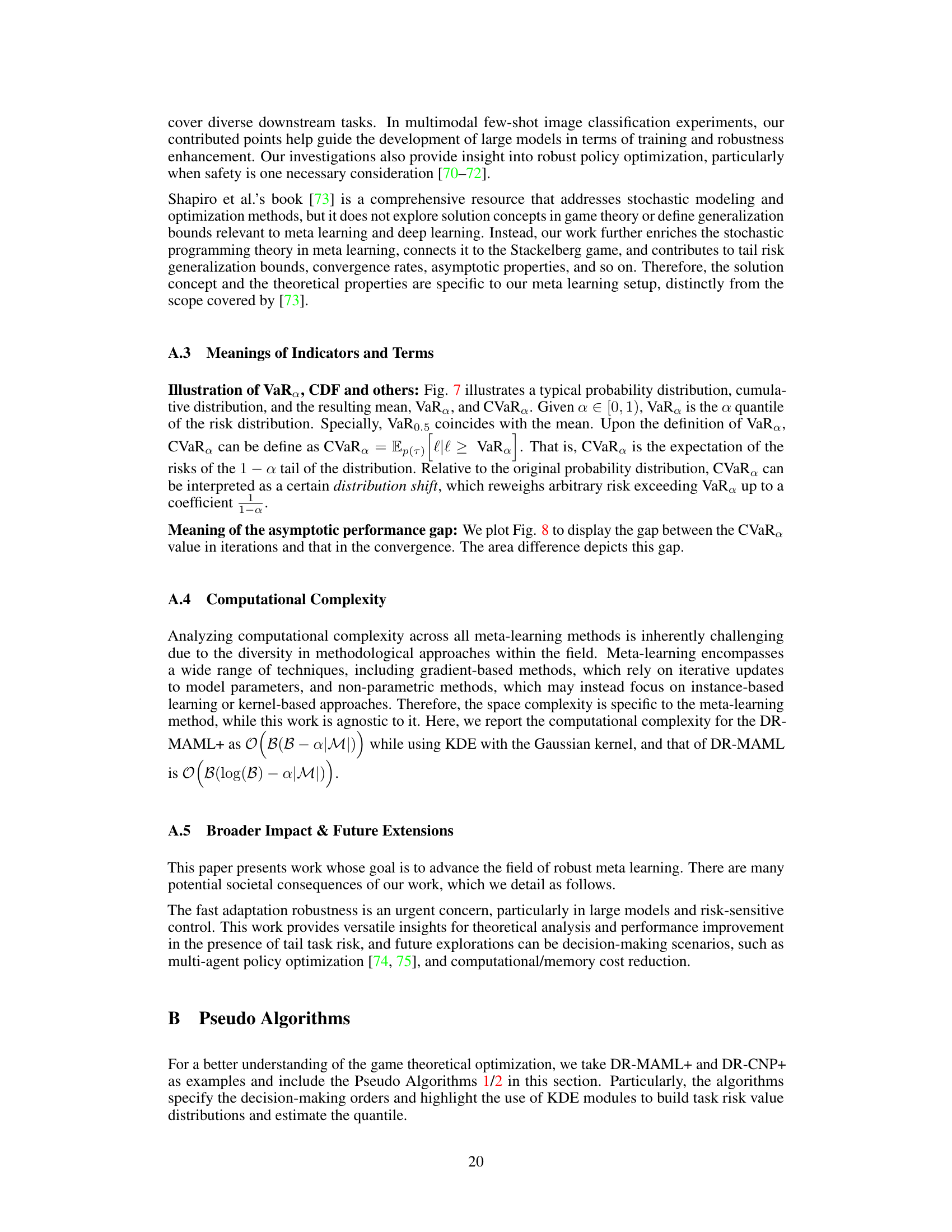
🔼 This figure compares the approximation errors of two methods for estimating the Value at Risk (VaR) - Monte Carlo (MC) and Kernel Density Estimation (KDE). The x-axis shows the size of the task batch used, representing the amount of data used in the approximation. The y-axis represents the absolute difference between the estimated VaR (from MC and KDE) and the true, or ‘Oracle,’ VaR. The plot demonstrates that KDE provides significantly more accurate VaR estimates, especially with smaller task batch sizes, indicating superior performance in scenarios with limited data.
read the caption
Figure 5: VaRa approximation errors with the crude MC and KDE. We compute the difference between the estimated VaR and the Oracle VaR in the absolute value |VaRa - VaR|.

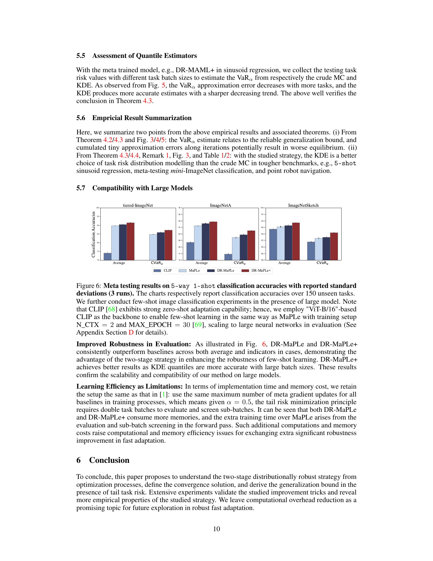
🔼 This figure compares the performance of different meta-learning methods (CLIP, MaPLe, DR-MaPLe, DR-MaPLe+) on three different few-shot image classification datasets (tiered-ImageNet, ImageNetA, ImageNetSketch). The results show classification accuracies (average and CVaR) across 150 unseen tasks for each method. DR-MaPLe+ consistently outperforms other methods, demonstrating the effectiveness of the proposed approach, particularly in achieving robustness.
read the caption
Figure 6: Meta testing results on 5-way 1-shot classification accuracies with reported standard deviations (3 runs). The charts respectively report classification accuracies over 150 unseen tasks. We further conduct few-shot image classification experiments in the presence of large model. Note that CLIP [68] exhibits strong zero-shot adaptation capability; hence, we employ \'ViT-B/16\'-based CLIP as the backbone to enable few-shot learning in the same way as MaPLe with training setup N_CTX = 2 and MAX_EPOCH = 30 [69], scaling to large neural networks in evaluation (See Appendix Section D for details).

🔼 This figure visually explains the concepts of risk in the context of fast adaptation. The x-axis represents the risk (l), and the y-axis shows both the probability density and the cumulative distribution function. The blue curve is the probability density function of the risk, while the red curve is the cumulative distribution function. The figure highlights the mean, VaRα (Value at Risk at level α), and CVaRα (Conditional Value at Risk at level α). The shaded area represents the tail risk beyond VaRα, and its area (after normalization by 1-α) represents CVaRα.
read the caption
Figure 7: Diagram of risk concepts in this work. Here, the x-axis is the task risk value in fast adaptation given a specific θ. The shadow-lined region illustrates the tail risk with a probability 1 – α in the probability density. The area of the shadow-lined region after 1 – α normalization corresponds to the expected tail risk CVaRa.

🔼 This figure illustrates the concept of the asymptotic performance gap in the bi-level optimization process of the distributionally robust meta-learning algorithm. It shows two distributions: one representing the optimal equilibrium (q*, θ*) and the other one representing an intermediate step (qT−1, θmeta). The dark blue area shows the distribution of task risk values at the equilibrium, while the light blue area highlights the difference between the intermediate and the equilibrium distributions. The sets T₁ and T₂ represent the tasks that contribute to the discrepancy between these two distributions. The figure visually explains how the algorithm iteratively approaches the Stackelberg equilibrium by reducing the difference between the two distributions.
read the caption
Figure 8: Illustration of the asymptotic behavior in approximating the equilibrium. Here, the x-axis is the feasible task risk value in fast adaptation. The dark blue region indicates the histogram of the task risk values in the local Stackelberg equilibrium (q*, θ*). The shallow blue region describes the histogram of the task risk values at some iterated point (qT-1, θmeta). The sets T₁ and T₂ respectively collect the tasks resulting the opposite order.

🔼 This figure illustrates the partitioning of the task space T into subsets based on the probability measures q1 and q2. The overlap between the subsets represents tasks that have non-zero probability in both q1 and q2.
read the caption
Figure 9: Partition of the task subspace. Here we take two probability measure {q1,q2} ∈ Qa for illustration. T₁ ∪ Tc and T₂ ∪ Tc defines the corresponding task subspaces for q1 and q2 with non-zero probability mass in the whole space T.

🔼 This figure shows four typical meta-learning benchmarks used in the paper’s experiments: (a) Sinusoid Regression, (b) System Identification, (c) Few-Shot Image Classification, and (d) Continuous Control. Each subfigure visually represents the task structure and data involved in the respective benchmark. The benchmarks are chosen to evaluate the performance of meta-learning models in various settings, testing their adaptability to diverse tasks and data characteristics.
read the caption
Figure 10: Typical meta learning benchmarks in evaluation.

🔼 This figure compares the performance of different meta-learning methods (MAML, TR-MAML, DRO-MAML, DR-MAML, and DR-MAML+) on a system identification task using 10-shot prediction. The histograms show the distributions of mean squared errors (MSEs) for each method. Lower MSEs indicate better performance. The figure also provides the average MSE and the Conditional Value at Risk (CVaR) for each method, offering a comprehensive view of the performance under both average and worst-case scenarios.
read the caption
Figure 11: Histograms of meta-testing performance in system identification. With α = 0.5, we visualize the comprision results of baselines and our DR-MAML+ in 10-shot prediction. The lower, the better for Average and CVaR values.
🔼 The figure shows the performance comparison of DR-MAML and DR-MAML+ under different confidence levels (alpha values) in the 5-shot sinusoid regression task. It compares the average, worst-case, and CVaR (Conditional Value-at-Risk) performance of the two models across various confidence levels. The shaded area represents the standard deviation. DR-MAML+ shows more stable performance across different confidence levels, highlighting the robustness provided by the use of the KDE method for quantile estimation, compared to the more volatile performance of the original DR-MAML method.
read the caption
Figure 12: Meta testing performance of DR-MAML and DR-MAML+ with different confidence level on Sinusoid 5-shot tasks. In the plots, the vertical axis is the MSEs, the horizontal axis is the confidence level, and the shaded area represents the standard deviation.

🔼 The figure shows the impact of different confidence levels on the performance of DR-MAML and DR-MAML+ in the sinusoid 5-shot regression task. Three subplots display the average, worst-case, and CVaR MSEs across various confidence levels. The shaded area in each subplot represents the standard deviation. It illustrates the relative robustness and stability of DR-MAML+ compared to DR-MAML across different confidence levels.
read the caption
Figure 13: Meta testing performance of DR-MAML and DR-MAML+ with different confidence level on Sinusoid 5-shot tasks. In the plots, the vertical axis is the MSEs, the horizontal axis is the confidence level, and the shaded area represents the standard deviation.

🔼 This figure displays the meta-testing performance of DR-MAML and DR-MAML+ on 5-shot sinusoid regression tasks using different confidence levels. The vertical axis represents the Mean Squared Error (MSE), and the horizontal axis represents the confidence level. Shaded areas indicate standard deviations, showing the variability in performance at each confidence level. The plots illustrate how performance varies across different evaluation metrics (Average, Worst, CVaR) as confidence level changes. This allows for a comparison of the two methods under varying levels of risk aversion.
read the caption
Figure 13: Meta testing performance of DR-MAML and DR-MAML+ with different confidence level on Sinusoid 5-shot tasks. In the plots, the vertical axis is the MSEs, the horizontal axis is the confidence level, and the shaded area represents the standard deviation.

🔼 This figure displays the risk landscapes for five different meta-learning methods (MAML, TR-MAML, DRO-MAML, DR-MAML, and DR-MAML+) on a 5-shot sinusoid regression task. Each landscape shows how the mean squared error (MSE) of the model’s fast adaptation varies depending on the amplitude (A) and phase (B) parameters of the sinusoidal function. It allows for a visual comparison of the robustness of each method to variations in the task parameters.
read the caption
Figure 15: The fast adaptation risk landscape of meta-trained MAML, TR-MAML, DRO-MAML, DR-MAML and DR-MAML+. The figure illustrates a 5-shot sinusoid regression example, mapping to the function space f(x) = A sin(x - B). The X-axis and Y-axis represent the amplitude parameter a and phase parameter b respectively. The plots exhibit testing MSEs on the Z-axis across random trials of task generation.
More on tables

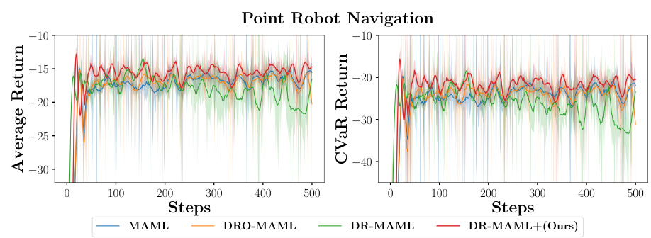
🔼 This table presents the results of meta-testing in a 2D point robot navigation task. Four runs were conducted with a confidence level of α = 0.5. The table compares the average return and the Conditional Value at Risk (CVaR) for several methods: MAML, DRO-MAML, DR-MAML, and the proposed DR-MAML+. The average return reflects the overall performance, while the CVaR indicates robustness to the worst-case scenarios.
read the caption
Table 2: Meta testing returns in point robot navigation (4 runs). The chart reports average return and CVaR return with α = 0.5.

🔼 This table compares several meta-learning methods focusing on their robustness to distributional shifts in the task space. It highlights key differences in the meta-learning objective function, whether generalization and convergence properties have been theoretically analyzed, and the type of robustness each method aims to achieve (e.g., worst-case robustness or robustness to tail risk). The table helps to contextualize the proposed DR-MAML+ method within the existing landscape of robust fast adaptation techniques.
read the caption
Table 3: A summary of robust fast adaptation methods. We take MAML as an example, list related methods, and report their characteristics in literature. We mainly report the statistics according to whether existing literature works include the generalization analysis and convergence analysis. The form of meta learner and the robustness type are generally connected.

🔼 This table shows the computational time and memory usage for three different methods: MaPLe, DR-MaPLe, and DR-MaPLe+. The baseline MaPLe’s time and memory are given, and the additional time and memory required by DR-MaPLe and DR-MaPLe+ are shown relative to MaPLe. This allows for comparison of the computational cost associated with each method.
read the caption
Table 4: Computational and memory cost in MaPLe relevant experiments.

🔼 This table presents the Mean Squared Errors (MSEs) for the Sinusoid 5-shot experiment, comparing different meta-learning methods. The results are averaged over five runs, and the best performance for each metric (Average, Worst, CVaRa) is highlighted in bold. The α value of 0.7 indicates the confidence level used for calculating the CVaRa (Conditional Value at Risk). The table showcases the performance of various methods in handling task distribution shifts, particularly focusing on robustness to tail risk events.
read the caption
Table 5: MSEs for Sinusoid 5-shot with reported standard deviations (5 runs). With α = 0.7, the best results are in bold.

🔼 This table presents the Mean Squared Errors (MSEs) for the Sinusoid 5-shot experiment across different methods. It compares the performance of various robust meta-learning approaches, including CNP, TR-CNP, DRO-CNP, DR-CNP, and the proposed DR-CNP+. The results are averaged over 5 runs, and the best performance for each metric (Average, Worst, and CVaRα) is highlighted in bold. The confidence level (α) used for the CVaRα calculation is 0.7. This table demonstrates the relative performance of different robustness strategies in handling tail risks in the task distribution.
read the caption
Table 5: MSEs for Sinusoid 5-shot with reported standard deviations (5 runs). With α = 0.7, the best results are in bold.

🔼 This table presents the average, worst-case, and CVaR mean squared errors (MSEs) for 5-shot and 10-shot sinusoid regression tasks. The results are based on five runs and cover 490 unseen test tasks. Lower MSE values indicate better performance. The bold values highlight the best-performing method for each metric.
read the caption
Table 7: Test average mean square errors (MSEs) with reported standard deviations for sinusoid regression (5 runs). We respectively consider 5-shot and 10-shot cases with α = 0.7. The results are evaluated across the 490 meta-test tasks, as in [42]. The best results are in bold.

🔼 This table presents the average 5-way 1-shot classification accuracies achieved by different meta-learning methods on the mini-ImageNet dataset. The results are reported with standard deviations, calculated over three runs. The table compares the performance of various methods under two different experimental setups, using eight meta-training tasks and four meta-testing tasks. The best results are highlighted in bold for each evaluation metric (Average, Worst, CVaRα). α = 0.5 represents the confidence level.
read the caption
Table 1: Average 5-way 1-shot classification accuracies in mini-ImageNet with reported standard deviations (3 runs). With a = 0.5, the best results are in bold.
Full paper#
