TL;DR#
Time series forecasting often struggles with managing channel interactions. Channel-independent (CI) strategies ignore crucial interactions while channel-dependent (CD) strategies can oversmooth data and reduce accuracy. Existing approaches poorly balance these aspects.
The proposed Channel Clustering Module (CCM) dynamically groups similar channels for improved forecasting, combining the strengths of CI and CD approaches. CCM boosts accuracy by an average 2.4% and 7.2% on long and short-term forecasting respectively, enables zero-shot forecasting, and improves model interpretability by uncovering intrinsic time series patterns among channels.
Key Takeaways#
Why does it matter?#
This paper is important because it introduces a novel and adaptable Channel Clustering Module (CCM) that significantly improves time series forecasting accuracy. CCM addresses the limitations of existing channel strategies by dynamically grouping similar channels, leading to better generalization and robustness. Its plug-and-play nature makes it readily applicable to various models, opening new avenues for research and development in time series forecasting.
Visual Insights#

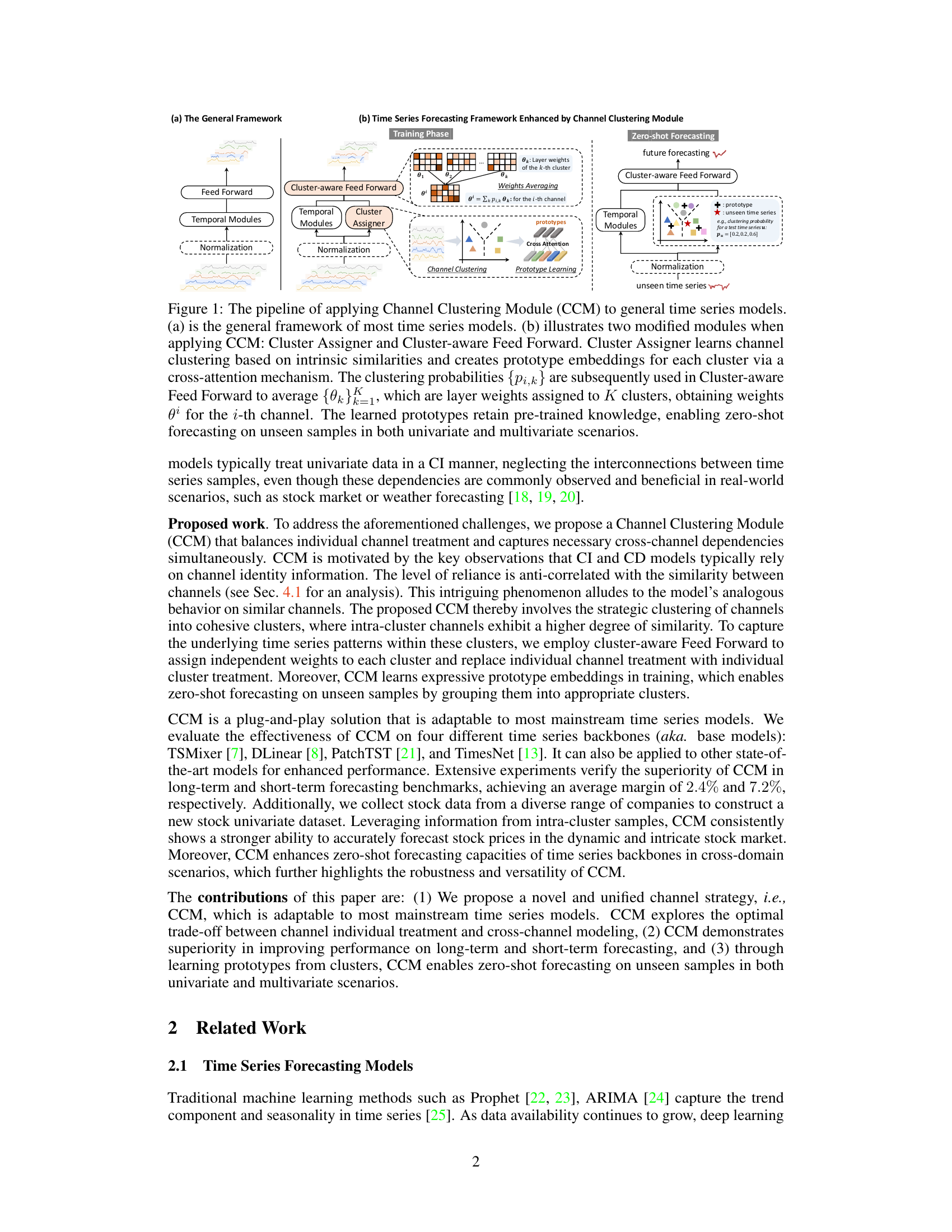
🔼 This figure shows the architecture of the Channel Clustering Module (CCM) for time series forecasting. Panel (a) depicts a general time series model framework, while panel (b) illustrates how CCM enhances this framework. CCM adds a ‘Cluster Assigner’ module that groups similar channels together based on their inherent similarities, learned via a cross-attention mechanism. The resulting cluster information is then used by the ‘Cluster-aware Feed Forward’ module to generate weights, effectively averaging the weights of channels within each cluster. The use of learned prototypes enables zero-shot forecasting on unseen time series data, meaning the model can make predictions on new channels without needing additional training.
read the caption
Figure 1: The pipeline of applying Channel Clustering Module (CCM) to general time series models. (a) is the general framework of most time series models. (b) illustrates two modified modules when applying CCM: Cluster Assigner and Cluster-aware Feed Forward. Cluster Assigner learns channel clustering based on intrinsic similarities and creates prototype embeddings for each cluster via a cross-attention mechanism. The clustering probabilities {pi,k} are subsequently used in Cluster-aware Feed Forward to average {0k}K_1, which are layer weights assigned to K clusters, obtaining weights θ for the i-th channel. The learned prototypes retain pre-trained knowledge, enabling zero-shot forecasting on unseen samples in both univariate and multivariate scenarios.
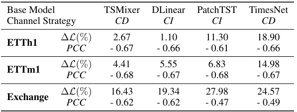
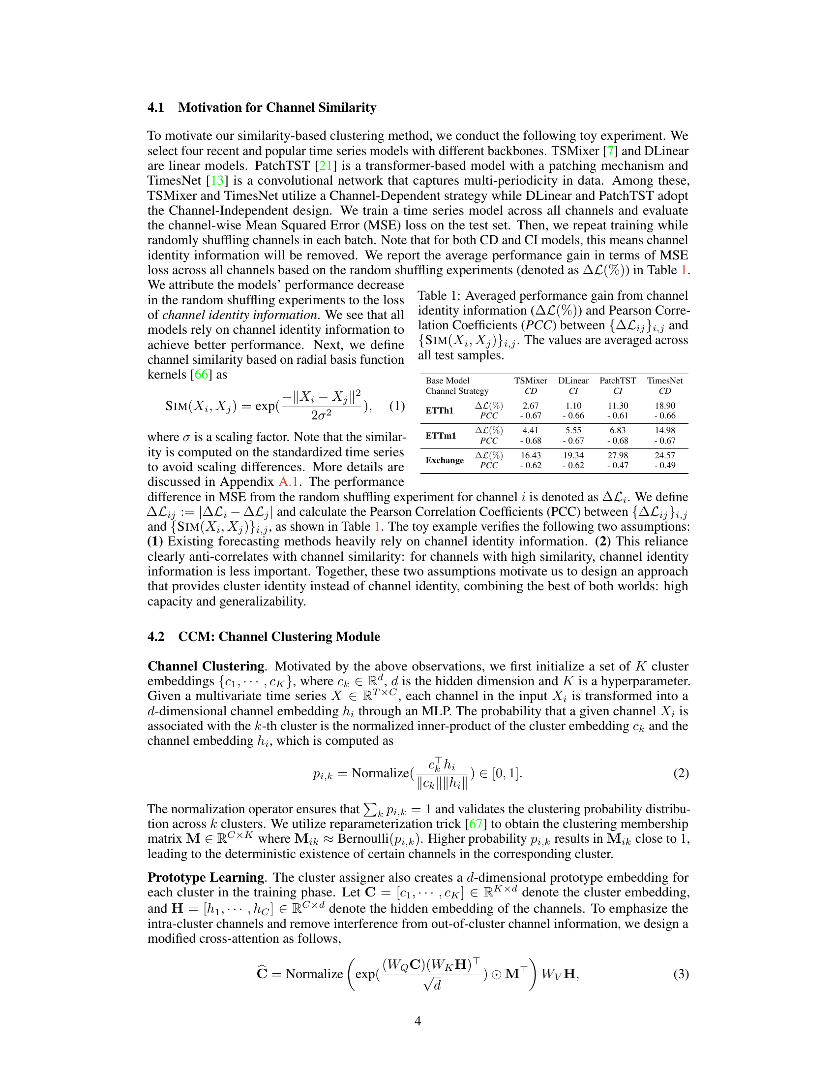
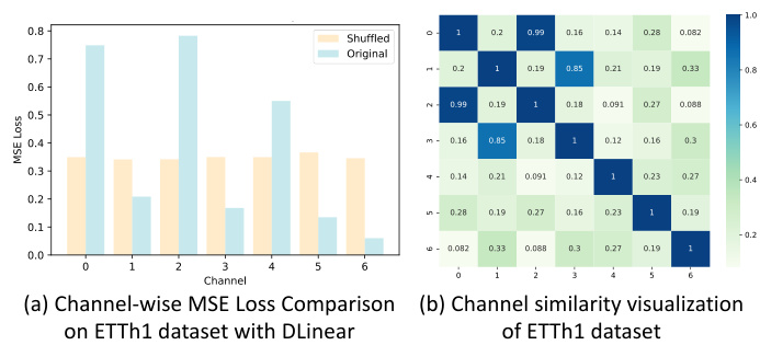
🔼 This table presents the results of a toy experiment designed to explore the relationship between channel similarity and model performance. Four different time series models (TSMixer, DLinear, PatchTST, TimesNet) with varying channel strategies (CD and CI) were trained. The performance was measured using MSE loss on test sets where channels were either kept in their original order or randomly shuffled. ∆L(%) represents the average performance gain (in terms of MSE loss) due to using the original channel order instead of randomly shuffling channels. The PCC (Pearson Correlation Coefficient) indicates the correlation between the performance gain and the calculated similarity between channel pairs using a radial basis function kernel. The negative PCC values indicate that the more similar the channels are, the less the model performance is affected by shuffling channels, suggesting the importance of channel identity.
read the caption
Table 1: Averaged performance gain from channel identity information (∆L(%)) and Pearson Correlation Coefficients (PCC) between {∆Lij}i,j and {SIM(Xi, Xj)}i,j. The values are averaged across all test samples.
In-depth insights#
Channel Similarity#
The concept of ‘Channel Similarity’ in time series forecasting is crucial for effectively leveraging information across multiple channels. High channel similarity suggests that the channels share underlying patterns or are intrinsically related, thus implying that combining information from these channels could improve forecasting accuracy by providing richer contextual information. Conversely, low channel similarity indicates that channels are distinct and independent, so attempting to combine them might lead to oversmoothing or worse performance. Therefore, understanding and quantifying channel similarity is key to deciding on the best channel strategy, whether it be a Channel-Independent (CI) or Channel-Dependent (CD) approach, or a hybrid method that selectively combines similar channels. A robust similarity metric is needed to accurately capture the relationships between channels and should be adaptable to different types of time series data and forecasting tasks. The effectiveness of any forecasting model heavily relies on making informed decisions on how to best integrate channel information, and a proper assessment of channel similarity plays a critical role in achieving this.
CCM Module#
The Channel Clustering Module (CCM) is a novel method for improving time series forecasting by dynamically grouping similar channels. CCM addresses the limitations of both Channel-Independent (CI) and Channel-Dependent (CD) strategies. CI methods, while achieving high performance on seen data, struggle with generalization to unseen data. CD methods, conversely, fail to capture individual channel characteristics effectively. CCM overcomes this by dynamically clustering channels based on their intrinsic similarities, allowing the model to leverage cluster-level information while still capturing individual channel dynamics. This approach is adaptable to most time series models, making it a versatile tool for enhancing forecasting accuracy and interpretability across diverse applications. CCM demonstrates significant performance improvements over existing CI and CD approaches, showcasing its effectiveness in both short-term and long-term forecasting scenarios. The ability of CCM to uncover underlying time series patterns and improve interpretability enhances understanding of complex systems, making it a valuable contribution to the field. Finally, CCM’s zero-shot forecasting capability, achieved through the learning of cluster prototypes, enables forecasting on unseen data, further strengthening its practical value.
Zero-shot Forecasting#
Zero-shot forecasting, a crucial aspect of time series prediction, tackles the challenge of forecasting unseen data without retraining the model. This capability is particularly valuable when dealing with limited data or when encountering novel data instances. The paper’s approach leverages pre-trained knowledge from existing clusters of similar time series. By clustering channels or time series based on inherent similarities, a model can generalize its learned patterns to new data points. This method mitigates the need for retraining on each new instance, enhancing efficiency and adaptability. The success hinges on the quality of the clustering algorithm and the representativeness of the existing clusters. Prototype learning, an integral part of the strategy, captures and stores the characteristics of each cluster, enabling efficient generalization to unseen data points that fall within existing clusters. This strategy significantly improves forecasting performance in cross-domain and cross-granularity scenarios, showcasing its versatility and robustness.
Ablation Studies#
Ablation studies systematically remove components of a model or process to understand their individual contributions. In the context of a time series forecasting model, ablation studies might involve removing the Channel Clustering Module (CCM), different loss functions, or varying the hyperparameters (like the number of clusters) to observe the effect on forecast accuracy. Such studies are critical for establishing causality and not just correlation, and provide insights into the model’s design choices. By analyzing the changes in model performance resulting from these removals, researchers gain a deeper understanding of which components are essential for good performance and which are redundant or even detrimental. This detailed analysis helps optimize model architecture and refine its capabilities, ultimately leading to more robust and efficient time series forecasts. Furthermore, a thorough ablation study strengthens the paper’s argument by supporting the rationale behind design decisions and demonstrating the specific value of the proposed methodologies.
Future Directions#
Future research should explore applying Channel Clustering Module (CCM) to diverse domains beyond time series forecasting, such as geospatial data analysis and biomedical signal processing, leveraging domain-specific knowledge to enhance the similarity computation. Dynamic clustering within CCM, adapting cluster assignments over time, warrants investigation to improve forecasting accuracy. Addressing the computational efficiency of CCM, particularly for large datasets and real-time applications, is crucial. Exploring alternative attention mechanisms to optimize CCM’s performance and scaling properties presents another vital area of future research. Finally, investigating the impact of CCM on various forecasting horizons and its effectiveness in different data settings with varying levels of noise and correlation is recommended to fully understand its capabilities and limitations.
More visual insights#
More on figures

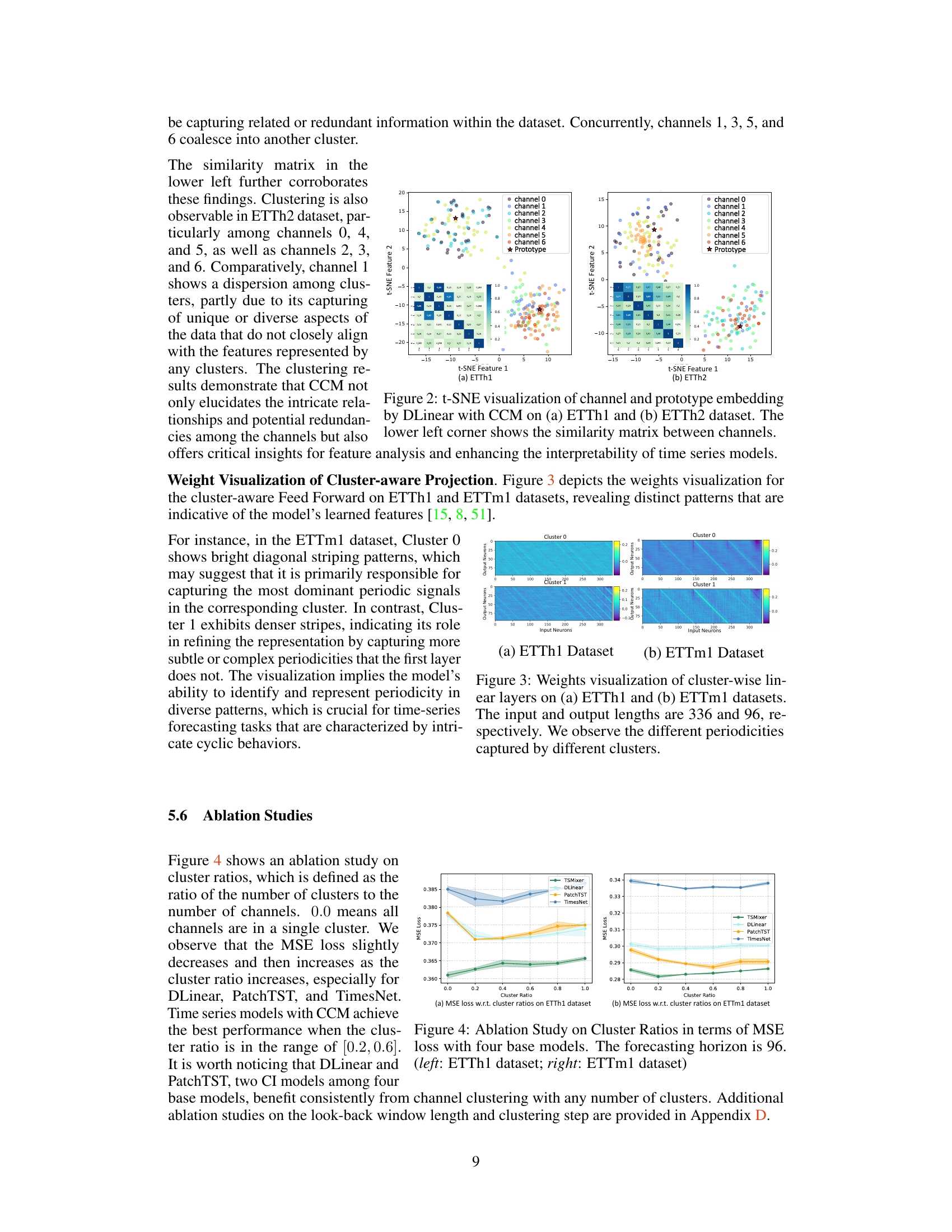
🔼 This figure visualizes the results of t-distributed Stochastic Neighbor Embedding (t-SNE) applied to channel and prototype embeddings generated by the DLinear model enhanced with the Channel Clustering Module (CCM). The left panel shows the results for the ETTh1 dataset, and the right panel shows the results for the ETTh2 dataset. Each point represents a channel within a sample. The color of each point indicates which channel the point represents. The black star represents the prototype. The lower-left corner of each panel displays a similarity matrix showing the similarity between each channel pair. The visualization demonstrates how CCM effectively groups similar channels together into clusters, indicating its ability to identify and leverage intra-cluster relationships within the data.
read the caption
Figure 2: t-SNE visualization of channel and prototype embedding by DLinear with CCM on (a) ETTh1 and (b) ETTh2 dataset. The lower left corner shows the similarity matrix between channels.
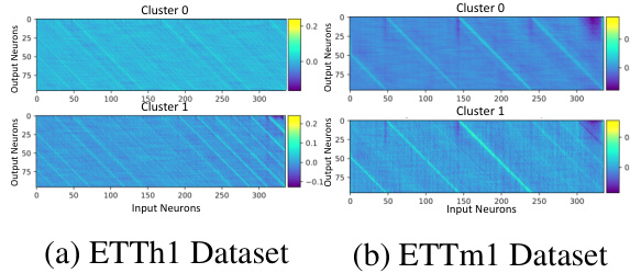
🔼 This figure visualizes the weights of the cluster-aware feed-forward layer in the Channel Clustering Module (CCM) for two datasets, ETTh1 and ETTm1. Each subfigure shows a heatmap representing the weights for each cluster (0 and 1). The heatmaps illustrate how the model learns different patterns within each cluster, suggesting that different clusters capture different periodicities in the time series data. The visualization provides insight into how CCM improves model interpretability by identifying distinct temporal patterns within clusters of channels.
read the caption
Figure 3: Weights visualization of cluster-wise linear layers on (a) ETTh1 and (b) ETTm1 datasets. The input and output lengths are 336 and 96, respectively. We observe the different periodicities captured by different clusters.
🔼 This figure shows the architecture of the Channel Clustering Module (CCM) and how it is integrated into a general time series forecasting model. Panel (a) depicts a standard time series model, while (b) illustrates the modifications made with CCM. The Cluster Assigner module groups similar channels together, creating prototype embeddings. The Cluster-aware Feed Forward then uses these embeddings to weight the contributions of each cluster to the final prediction, improving both performance and allowing for zero-shot forecasting on unseen data.
read the caption
Figure 1: The pipeline of applying Channel Clustering Module (CCM) to general time series models. (a) is the general framework of most time series models. (b) illustrates two modified modules when applying CCM: Cluster Assigner and Cluster-aware Feed Forward. Cluster Assigner learns channel clustering based on intrinsic similarities and creates prototype embeddings for each cluster via a cross-attention mechanism. The clustering probabilities {pi,k} are subsequently used in Cluster-aware Feed Forward to average {0k}K_1, which are layer weights assigned to K clusters, obtaining weights θ for the i-th channel. The learned prototypes retain pre-trained knowledge, enabling zero-shot forecasting on unseen samples in both univariate and multivariate scenarios.
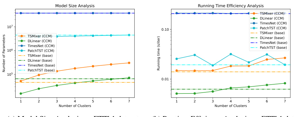
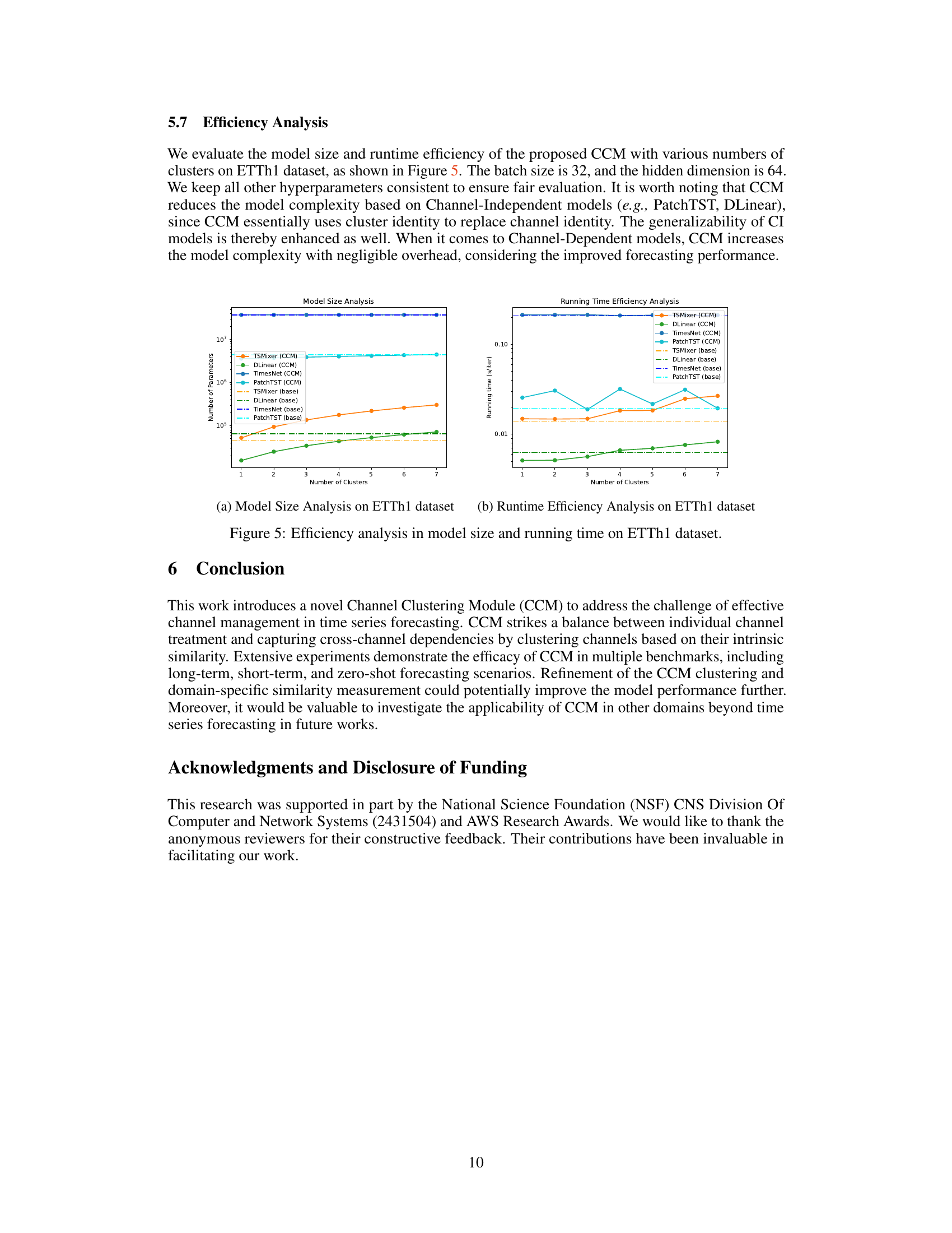
🔼 This figure shows the model size and running time efficiency of the proposed CCM with various numbers of clusters on the ETTh1 dataset. The left panel displays the number of parameters for the base models (TSMixer, DLinear, TimesNet, PatchTST) and their CCM-enhanced counterparts as a function of the number of clusters. The right panel illustrates the running time (in seconds per iteration) for the same models. The plots reveal that CCM reduces model size for Channel-Independent models and introduces negligible overhead for Channel-Dependent models, while maintaining or improving efficiency.
read the caption
Figure 5: Efficiency analysis in model size and running time on ETTh1 dataset.
🔼 This figure visualizes the results of t-SNE dimensionality reduction applied to channel and prototype embeddings generated by the Channel Clustering Module (CCM) enhanced DLinear model. The visualization helps understand the inherent relationships and groupings of channels within the ETTh1 and ETTh2 datasets. Panel (a) shows the ETTh1 dataset visualization and panel (b) shows the ETTh2 dataset visualization. The lower-left corner of each panel displays a similarity matrix, providing a quantitative measure of the relationships between channels.
read the caption
Figure 2: t-SNE visualization of channel and prototype embedding by DLinear with CCM on (a) ETTh1 and (b) ETTh2 dataset. The lower left corner shows the similarity matrix between channels.
More on tables
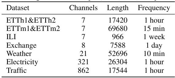
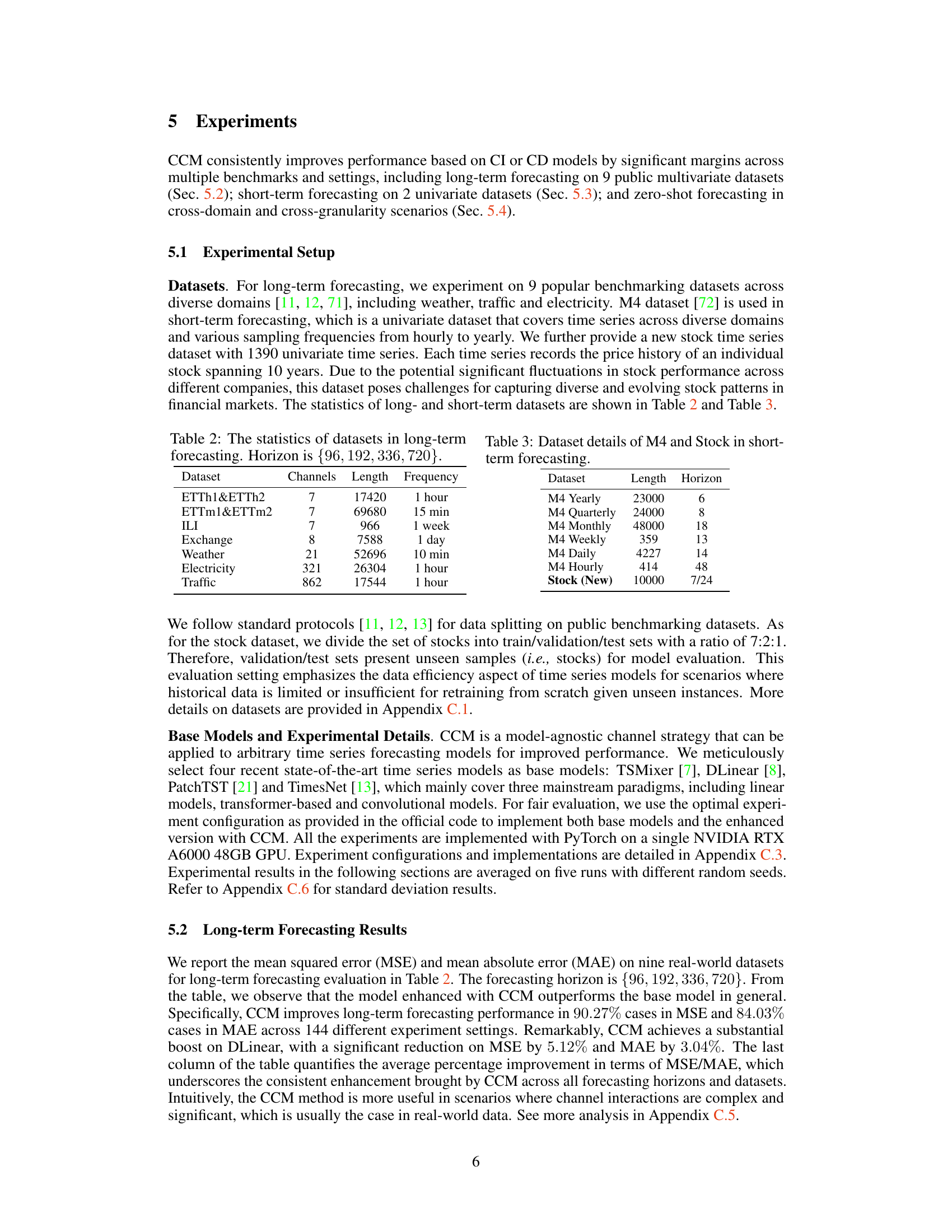
🔼 This table presents the characteristics of nine datasets used for long-term time series forecasting experiments in the paper. For each dataset, it lists the number of channels (variates), the length of the time series (number of data points), the frequency of data sampling, and the forecasting horizons used in the experiments. The datasets cover diverse domains including weather, traffic, electricity, and illness data, offering a comprehensive benchmark for evaluating the proposed method.
read the caption
Table 2: The statistics of datasets in long-term forecasting. Horizon is {96, 192, 336, 720}.
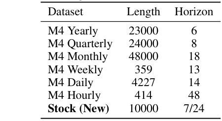
🔼 This table presents the length and horizon of the time series datasets used for short-term forecasting. The M4 dataset is broken down by the frequency of the time series (Yearly, Quarterly, Monthly, Weekly, Daily, Hourly), showing the number of data points (length) and the prediction time range (horizon) for each. A new Stock dataset is also included, which has 10,000 time series and a horizon of 7 or 24, depending on the experiment setup.
read the caption
Table 3: Dataset details of M4 and Stock in short-term forecasting.
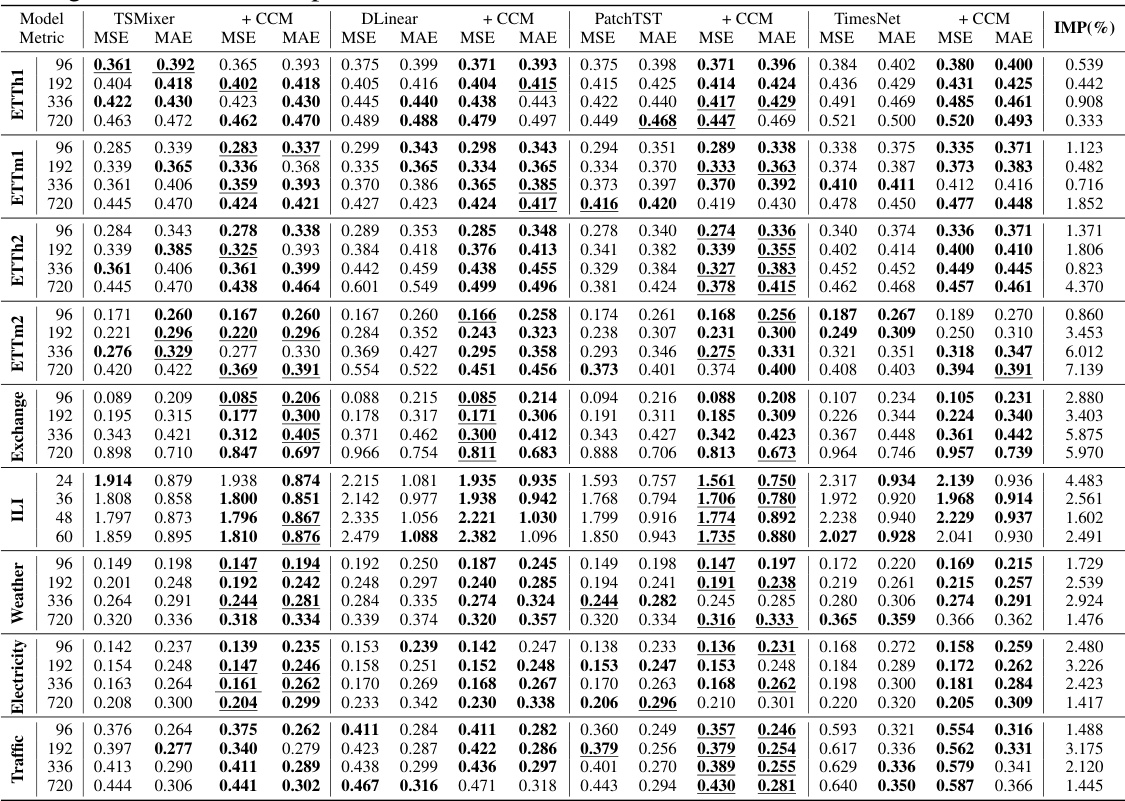
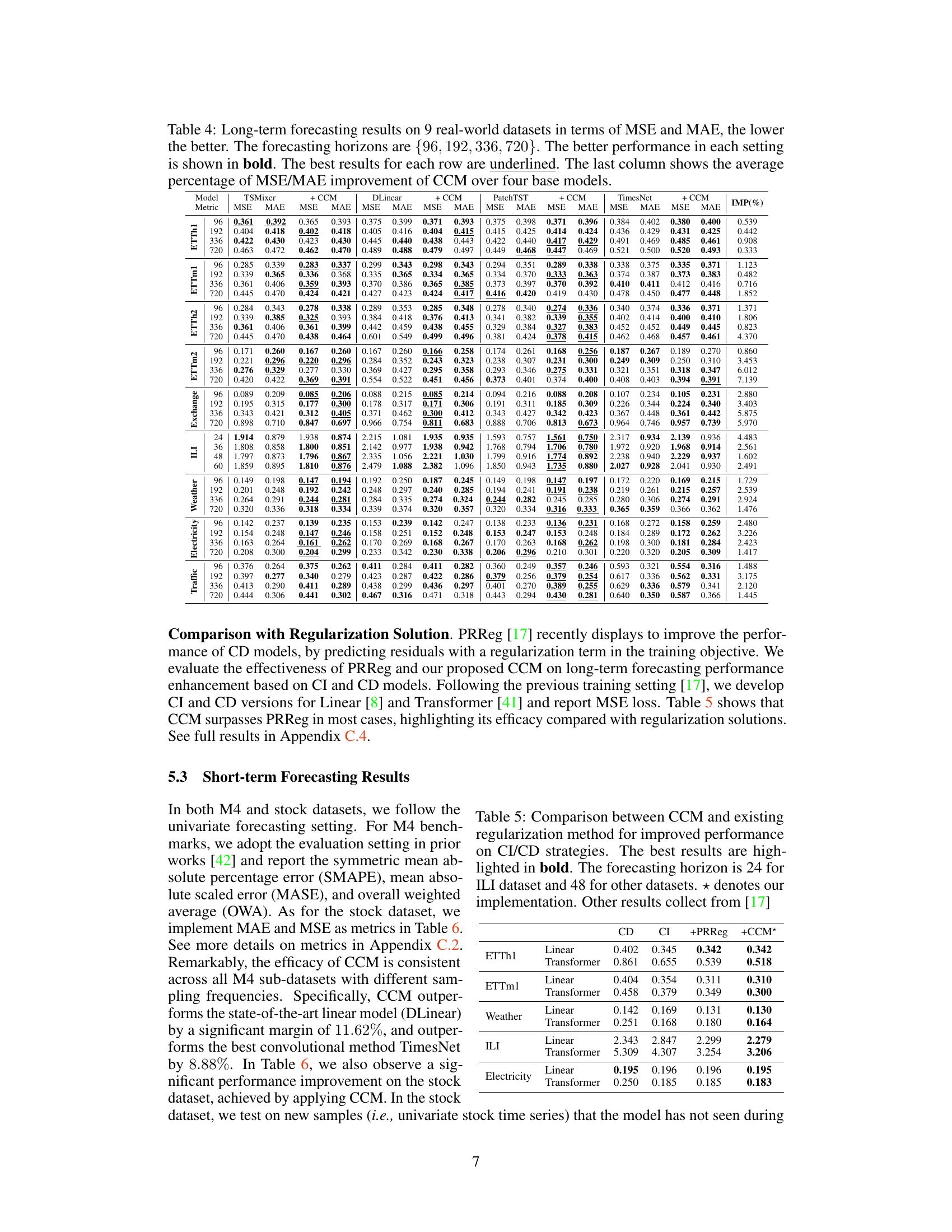
🔼 This table presents the results of long-term time series forecasting experiments on nine real-world datasets using four different base models (TSMixer, DLinear, PatchTST, TimesNet) with and without the Channel Clustering Module (CCM). The table shows the Mean Squared Error (MSE) and Mean Absolute Error (MAE) for each model and dataset at four different forecasting horizons (96, 192, 336, and 720 time steps). The best performing model for each row is underlined and the percentage improvement achieved by CCM over the four base models is given in the last column. Lower MSE and MAE values indicate better forecasting performance.
read the caption
Table 4: Long-term forecasting results on 9 real-world datasets in terms of MSE and MAE, the lower the better. The forecasting horizons are {96, 192, 336, 720}. The better performance in each setting is shown in bold. The best results for each row are underlined. The last column shows the average percentage of MSE/MAE improvement of CCM over four base models.
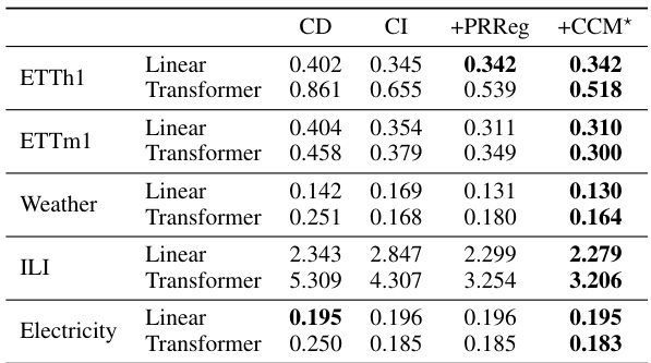
🔼 This table compares the performance of the proposed Channel Clustering Module (CCM) against a previously published regularization method (PRReg) for improving the performance of Channel-Independent (CI) and Channel-Dependent (CD) models in time series forecasting. The metric used is Mean Squared Error (MSE), and lower values indicate better performance. The table shows that for various datasets (ETTh1, ETTm1, Weather, ILI, Electricity), CCM generally outperforms or matches PRReg in terms of MSE reduction across different model types (linear and transformer).
read the caption
Table 5: Comparison between CCM and existing regularization method for improved performance on CI/CD strategies in terms of MSE metric. The best results are highlighted in bold.

🔼 This table presents the results of long-term forecasting experiments conducted on nine real-world datasets using four different time series forecasting models: TSMixer, DLinear, PatchTST, and TimesNet. Each model was evaluated with and without the Channel Clustering Module (CCM). The table displays the Mean Squared Error (MSE) and Mean Absolute Error (MAE) for each model and dataset across four different forecasting horizons (96, 192, 336, and 720). The best performing model for each horizon and dataset is highlighted in bold, and the best overall result for each row is underlined. The final column shows the average percentage improvement in MSE and MAE achieved by CCM across all models and datasets.
read the caption
Table 4: Long-term forecasting results on 9 real-world datasets in terms of MSE and MAE, the lower the better. The forecasting horizons are {96, 192, 336, 720}. The better performance in each setting is shown in bold. The best results for each row are underlined. The last column shows the average percentage of MSE/MAE improvement of CCM over four base models.

🔼 This table presents the results of zero-shot forecasting experiments conducted on the ETT datasets. The model was trained on one subset of the ETT data and then tested on unseen subsets (ETTh1 to ETTh2, ETTh1 to ETTm1, etc.). Two different forecasting horizons were used (96 and 720). The table shows the Mean Squared Error (MSE) and Mean Absolute Error (MAE) for each model and generalization task. The best performing model for each row is underlined. The purpose is to demonstrate the effectiveness of the proposed method (CCM) in scenarios where the model must generalize to unseen data.
read the caption
Table 7: Zero-shot forecasting results on ETT datasets. The forecasting horizon is {96, 720}. The best value in each row is underlined.

🔼 This table shows the time complexity of different similarity computation approaches used in the paper. The time complexity is expressed in Big O notation and depends on the length (H) of the time series. Euclidean distance has a time complexity of O(H), while Edit Distance, Dynamic Time Warping (DTW), Longest Common Subsequence (LCSS), and Cross-correlation (CCor) all have a time complexity of O(H^2).
read the caption
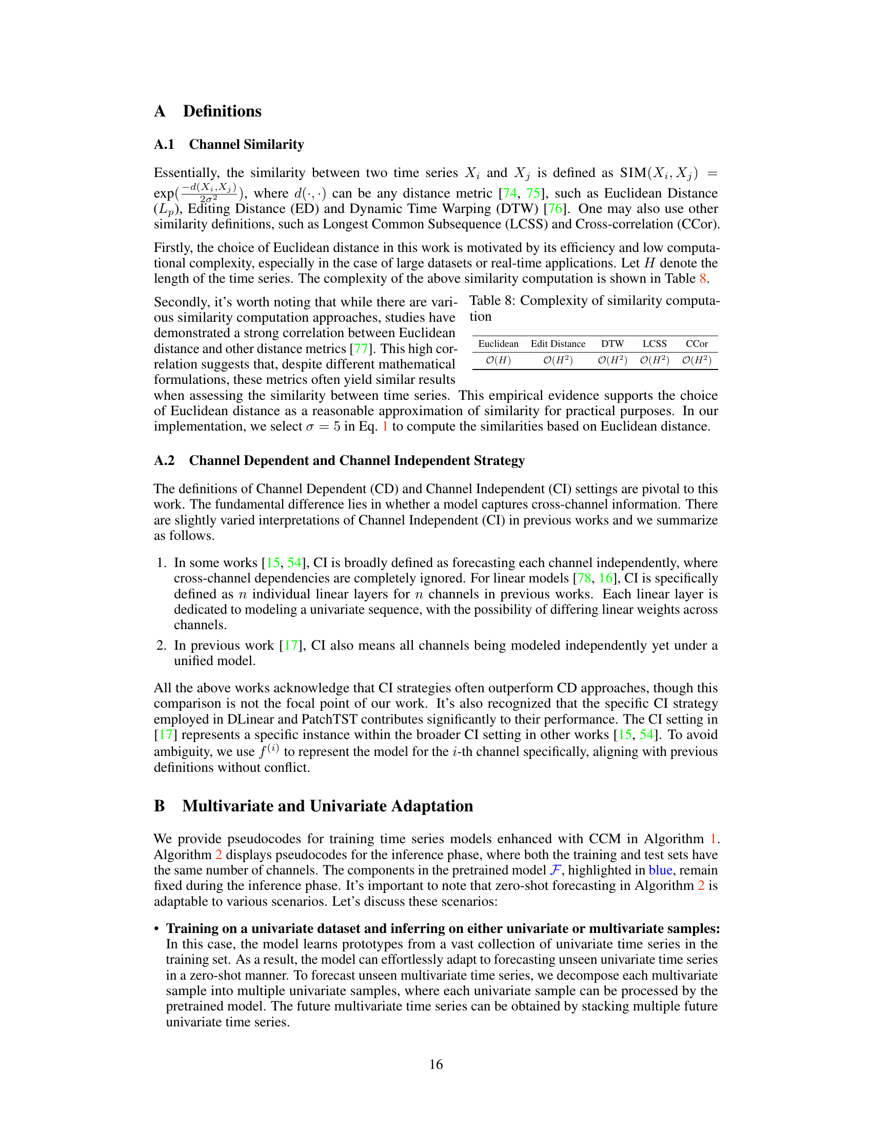
Table 8: Complexity of similarity computation

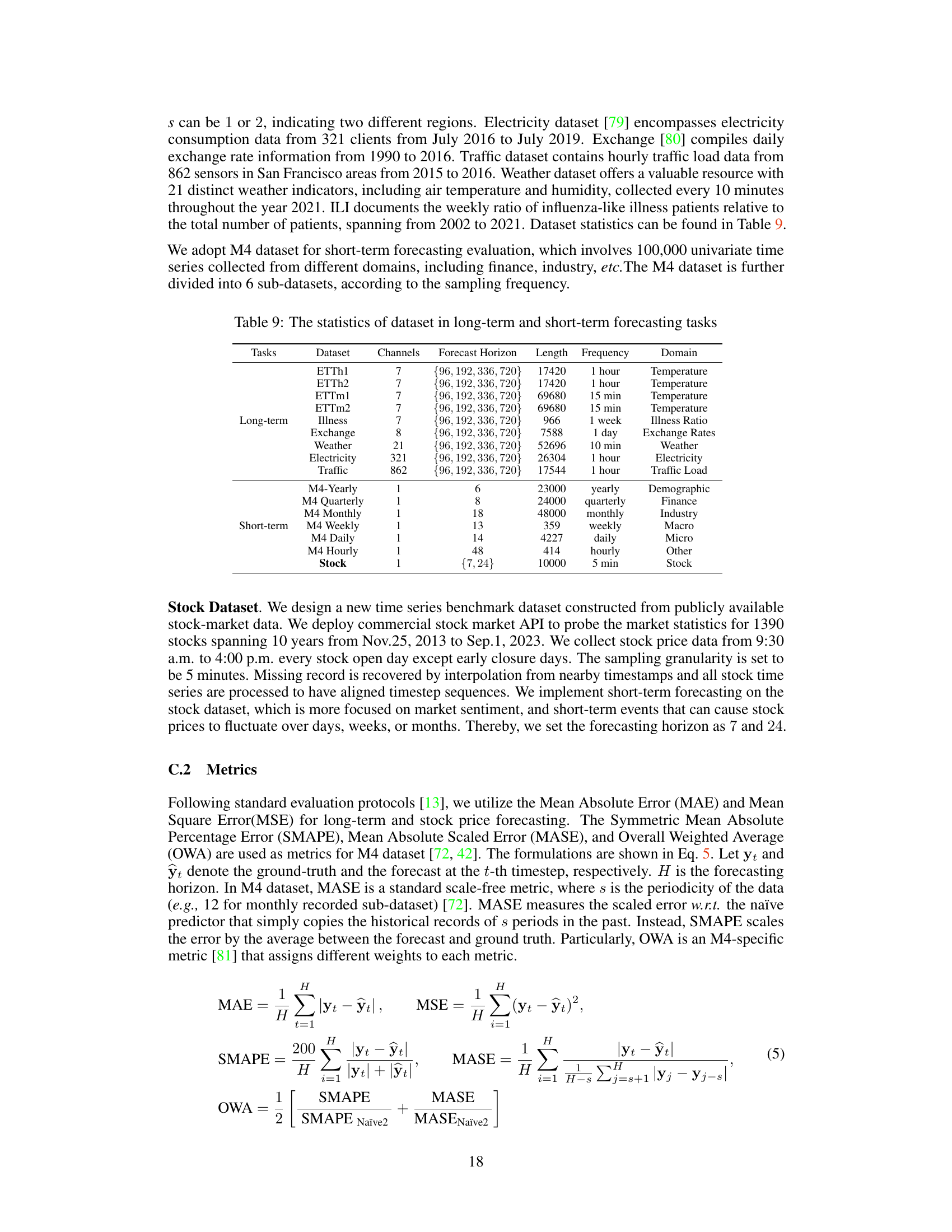
🔼 This table presents the characteristics of the datasets used in the paper’s experiments. It shows the dataset name, number of channels, forecasting horizon (the number of future time steps to predict), the length of the time series, the frequency of data points (e.g., hourly, daily, etc.), and the domain from which the data originates. It’s divided into long-term and short-term forecasting tasks, which reflects the different prediction horizons used in the respective experiments.
read the caption
Table 9: The statistics of dataset in long-term and short-term forecasting tasks

🔼 This table shows the hyperparameters used in the experiments for different datasets. It includes the number of clusters (K) used in the Channel Clustering Module (CCM), the regularization parameter (β), the number of linear layers in the MLP for channel embedding, the hidden dimension of the embedding, and the number of layers in each of the four base time series models (TSMixer, DLinear, PatchTST, TimesNet). The values are optimized for each dataset.
read the caption
Table 10: Experiment configuration.

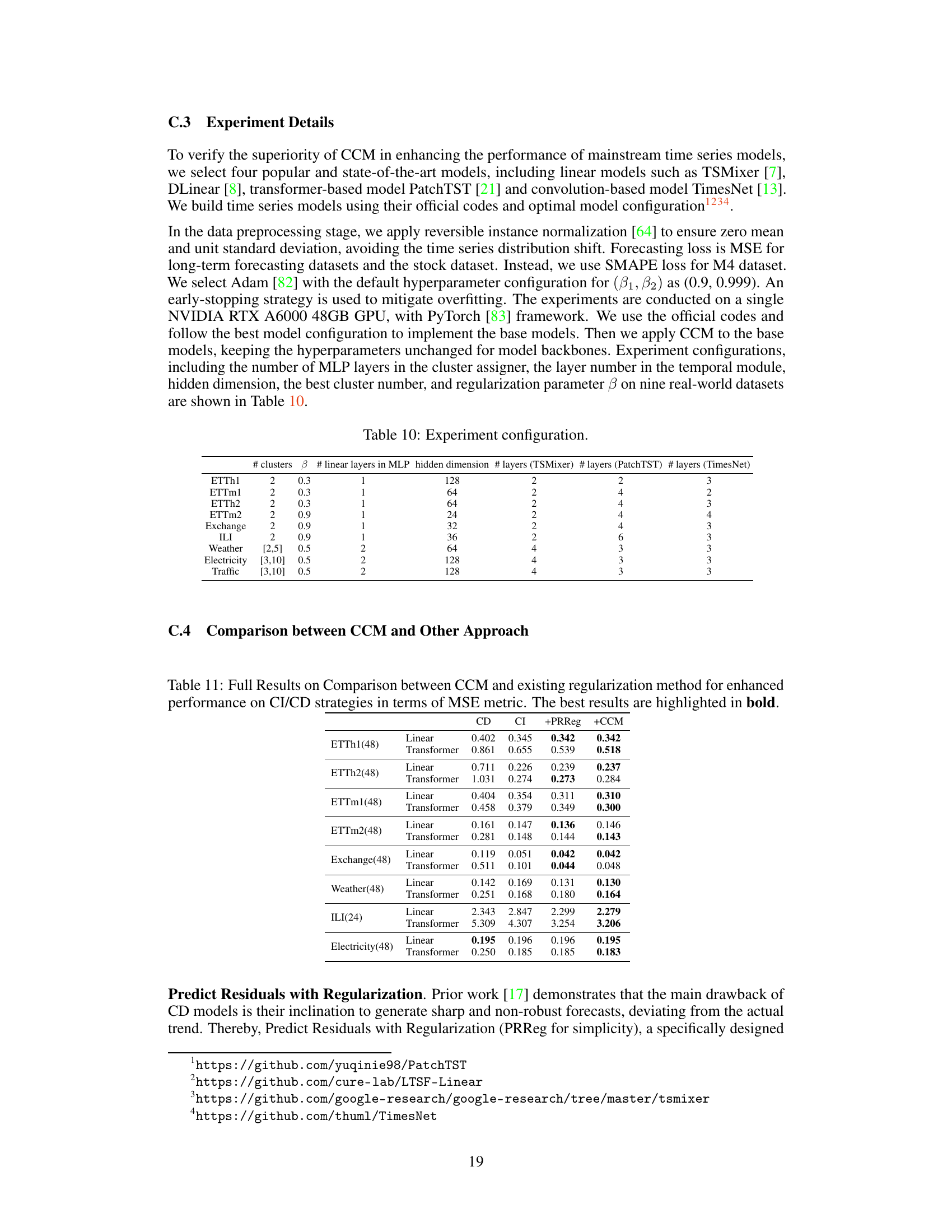
🔼 This table compares the performance of the proposed Channel Clustering Module (CCM) against the Channel Independent (CI) and Channel Dependent (CD) strategies, as well as a previously proposed regularization method (PRReg). The results, measured by MSE (Mean Squared Error), are presented for multiple datasets and different model types (Linear and Transformer). The table shows CCM’s ability to improve performance on both CI and CD baselines.
read the caption
Table 11: Full Results on Comparison between CCM and existing regularization method for enhanced performance on CI/CD strategies in terms of MSE metric. The best results are highlighted in bold.

🔼 This table shows the average Pearson correlation coefficient (r) among channels for each of the nine datasets used in the long-term forecasting experiments. The correlation coefficient is a measure of the linear relationship between channels, ranging from -1 (perfect negative correlation) to +1 (perfect positive correlation). A value of 0 indicates no linear correlation. This table provides insight into the inherent relationships between channels within each dataset, which influences the effectiveness of different channel strategies (Channel-Independent vs. Channel-Dependent).
read the caption
Table 12: Multivariate intrinsic similarity for long-term forecasting datasets

🔼 This table presents the average Pearson correlation coefficients (r) between time series in different M4 sub-datasets (Yearly, Quarterly, Monthly, Weekly, Daily, Hourly). It shows the degree of multivariate correlation across channels in the datasets, which is used to assess the influence of intrinsic similarity on forecasting performance. Higher correlation indicates stronger inherent relationships between time series within the dataset.
read the caption
Table 13: Intrinsic similarity for short-term forecasting datasets

🔼 This table shows the standard deviation of the MSE and MAE values reported in Table 2 for nine real-world datasets used in long-term forecasting experiments. The forecasting horizon for all experiments was 96 time steps. The table provides a measure of the variability in the model’s performance across multiple runs with different random seeds for each dataset and model configuration. It helps to understand the reliability of the results presented in Table 2.
read the caption
Table 14: Standard deviation of Table 2 on long-term forecasting benchmarks. The forecasting horizon is 96.
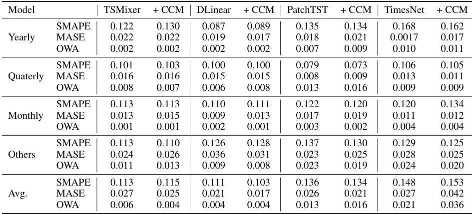
🔼 This table presents the results of short-term forecasting experiments using four different time series models (TSMixer, DLinear, PatchTST, TimesNet) with and without the Channel Clustering Module (CCM). The models are evaluated on the M4 dataset (with yearly, quarterly, monthly, weekly, daily, and hourly sub-datasets) and a new stock dataset. The metrics used are SMAPE, MASE, and OWA for the M4 dataset, and MSE and MAE for the stock dataset. The table shows the performance of each model for different forecasting horizons (7 and 24 for the stock dataset), highlighting the best-performing model in each case.
read the caption
Table 6: Short-term forecasting results on M4 dataset in terms of SMAPE, MASE, and OWA, and stock dataset in terms of MSE and MAE. The lower the better. The forecasting horizon is {7, 24} for the stock dataset. The better performance in each setting is shown in bold.

🔼 This table presents the standard deviations of the MSE and MAE metrics reported in Table 6 for the stock dataset. It shows the variability in performance across multiple runs for different models (TSMixer, DLinear, PatchTST, TimesNet) with and without the Channel Clustering Module (CCM), for both forecasting horizons (7 and 24). The low standard deviations indicate consistent performance across runs.
read the caption
Table 16: Standard deviation of Table 6 on stock dataset
🔼 This table presents the results of a toy experiment designed to motivate the concept of channel similarity. The experiment randomly shuffles channels within batches during training, removing channel identity information. The table shows the average performance drop (∆L(%)) for four different time series models, each using either a channel-dependent (CD) or channel-independent (CI) strategy. It also presents the Pearson Correlation Coefficient (PCC) between the performance drop and the channel similarity (SIM(Xi, Xj)) calculated using radial basis function kernels. The negative PCC values indicate an anticorrelation between channel similarity and the impact of shuffling, supporting the hypothesis that the model’s reliance on channel identity information is inversely proportional to the similarity between channels.
read the caption
Table 1: Averaged performance gain from channel identity information (∆L(%)) and Pearson Correlation Coefficients (PCC) between {∆Lij}i,j and {SIM(Xi, Xj)}i,j. The values are averaged across all test samples.

🔼 This table presents the results of short-term stock price forecasting experiments using different look-back window lengths (14, 21, 28). The forecasting horizon is 7 days. The table compares the Mean Squared Error (MSE) and Mean Absolute Error (MAE) for four different time series forecasting models (TSMixer, DLinear, PatchTST, TimesNet), both with and without the Channel Clustering Module (CCM). The best-performing model for each configuration is underlined, and bold values indicate cases where CCM improved performance compared to the baseline model. The ‘Imp.’ column shows the percentage improvement achieved by CCM. The results highlight the impact of different look-back window lengths on forecasting accuracy and the effectiveness of CCM in improving performance.
read the caption
Table 18: Short-term forecasting on stock dataset with different look-back window length in {14,21,28}. The forecasting length is 7. The best results with the same base model are underlined. Bold means CCM successfully enhances forecasting performance over the base model.

🔼 This table compares the performance of the proposed Channel Clustering Module (CCM) against a previously proposed regularization method (PRReg) for improving the performance of Channel-Independent (CI) and Channel-Dependent (CD) models in time series forecasting. The results are presented in terms of Mean Squared Error (MSE), a common metric for evaluating forecasting accuracy. Lower MSE values indicate better performance. The table shows that CCM generally outperforms PRReg across different model types (Linear and Transformer) and datasets (ETTh1, ETTm1, Weather, ILI, Electricity).
read the caption
Table 5: Comparison between CCM and existing regularization method for improved performance on CI/CD strategies in terms of MSE metric. The best results are highlighted in bold.
Full paper#

