TL;DR#
Many real-world clustering problems require optimizing multiple, often conflicting, objectives. This paper tackles the challenge of bi-objective k-clustering, where two objectives (e.g., minimizing cluster diameter and maximizing inter-cluster separation) must be balanced. Existing approaches often simplify the problem by focusing on a weighted sum or constrained optimization, potentially overlooking good solutions. This work addresses these limitations by focusing on the Pareto front, which represents the set of optimal trade-offs.
The paper develops novel algorithms to approximate the Pareto front for various combinations of bi-objective clustering problems, including k-center, k-diameter, k-median, k-means, and k-separation. These algorithms offer provable approximation guarantees, demonstrating theoretical soundness. Extensive experiments validate the approach’s practical effectiveness, showcasing its ability to discover high-quality clusterings unattainable by traditional methods. The findings highlight the advantages of using the Pareto-optimal solutions for improved data analysis and visualization.
Key Takeaways#
Why does it matter?#
This paper is crucial for researchers in multi-objective optimization and clustering because it provides novel algorithms with provable approximation guarantees for finding Pareto-optimal solutions in bi-objective clustering problems. It addresses a significant gap in the field by handling conflicting objectives and offers a more comprehensive and flexible approach than traditional single-objective methods. The results are also applicable to other multi-criteria optimization problems and open up new avenues for research in visualization and data analysis.
Visual Insights#

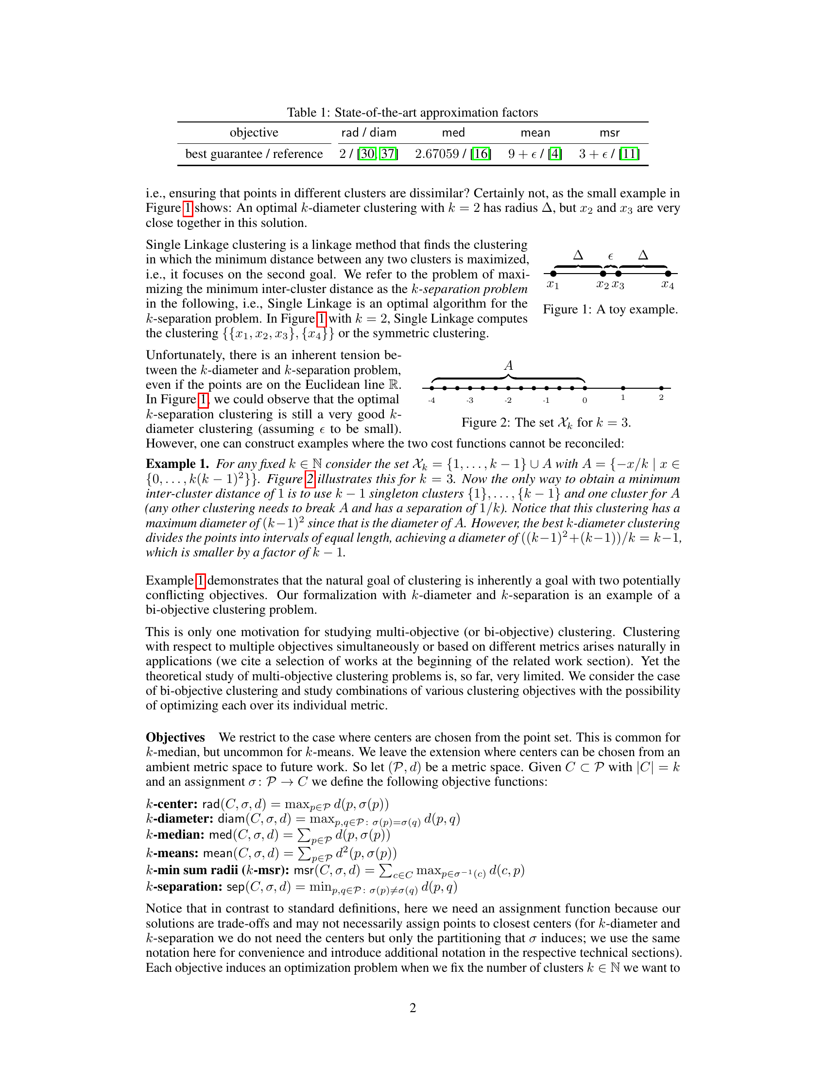
🔼 This figure shows a simple example of a point set in one dimension, illustrating the tension between the k-diameter and k-separation problems in clustering. An optimal k-diameter clustering (minimizing the maximum diameter of any cluster) with k=2 might result in clusters where points in different clusters are quite close together. Conversely, an optimal k-separation clustering (maximizing the minimum distance between clusters) could result in clusters that are less compact in terms of diameter. This highlights the conflicting nature of these two objectives in clustering.
read the caption
Figure 1: A toy example.

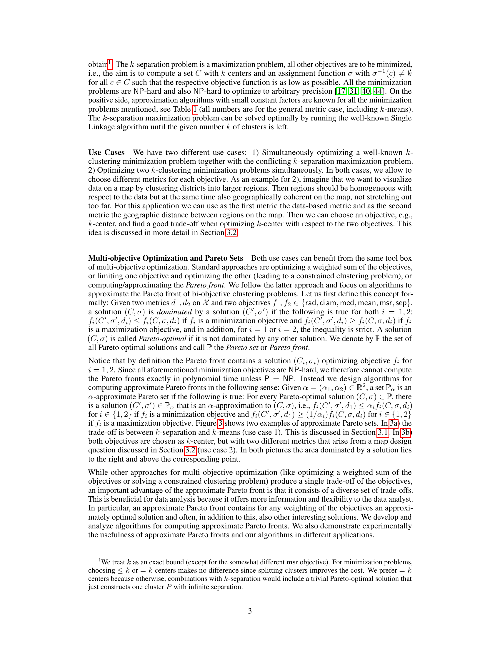
🔼 This table shows the best known approximation guarantees for various k-clustering objectives (k-center, k-diameter, k-median, k-means, k-min sum radii). The approximation factors represent the worst-case performance ratio of an algorithm compared to the optimal solution. For example, a factor of 2 for k-center/k-diameter means that the algorithm’s solution is at most twice as bad as the optimal solution.
read the caption
Table 1: State-of-the-art approximation factors
In-depth insights#
Pareto Front Approx#
Approximating the Pareto front efficiently is crucial for multi-objective optimization problems, particularly in computationally expensive domains like clustering. A thoughtful approach to Pareto front approximation balances accuracy with computational tractability. The core idea is to design algorithms that guarantee finding a set of solutions within a provable distance (an approximation factor) of the true Pareto front. This involves carefully selecting algorithms for individual objectives and strategically combining their outputs to create a representative subset of the Pareto-optimal solutions. The choice of approximation algorithms is critical, as they determine both the accuracy and efficiency of the overall process. Different combinations of objectives will necessitate different algorithmic approaches. The paper likely explored various techniques for combining these approximated solutions, potentially including weighted sums, constraint optimization, or other more sophisticated methods. Experimental validation is essential to demonstrate the effectiveness of the proposed approximation scheme in practice. The analysis should ideally compare the generated approximate Pareto front to the true Pareto front (if computable) and analyze the trade-off between solution quality and computational cost. The generated approximate Pareto front should contain high-quality clustering solutions that are not obtainable by optimizing single objectives alone.
Bi-objective Clusters#
Bi-objective clustering tackles the challenge of optimizing multiple, often conflicting, objectives simultaneously. Instead of seeking a single “best” clustering, it aims to identify a set of Pareto-optimal solutions, representing different trade-offs between the objectives. This approach is particularly useful when dealing with real-world problems where a single objective might not capture the full complexity of the desired outcome. For instance, a data visualization task may require both geographically compact and thematically homogeneous clusters; a balance between these is crucial, but difficult to achieve with a single objective function. A key advantage is the exploration of the solution space, revealing diverse clustering structures that might be missed by single-objective methods. The resulting Pareto front allows for a more informed decision, providing flexibility to select the clustering that best meets the specific needs of the application. Developing efficient algorithms to approximate the Pareto front for different combinations of objectives is a major challenge in bi-objective clustering research. This involves dealing with computational complexity and providing approximation guarantees. The process requires novel algorithmic designs to efficiently handle the trade-offs between objectives and produce meaningful results.
Multi-metric Methods#
Multi-metric methods in clustering aim to leverage the strengths of diverse distance metrics to capture richer data representations. Instead of relying on a single metric, which may fail to capture the complexity of relationships within data, these methods integrate multiple metrics, often combining them in sophisticated ways. This could involve using different metrics for different objectives (e.g., spatial proximity and feature similarity), weighting metrics based on their relevance to specific aspects of the data, or dynamically switching between metrics based on data characteristics. The key challenge is managing the inherent conflicts that may arise when using multiple, potentially contradictory metrics. Effective techniques often employ multi-objective optimization to find Pareto-optimal solutions that balance the trade-offs between different metrics, allowing for a more nuanced and insightful understanding of the data’s structure. The result is often a more robust and accurate clustering that reflects the multifaceted nature of the data more effectively than methods limited to a single metric. Approximation algorithms and heuristic approaches are frequently employed because the problem is computationally complex, especially as the number of metrics and data points increase. The selection of appropriate metrics and their combination strategy is crucial, requiring a careful consideration of data properties and analytical goals. Therefore, effective visualizations are vital for understanding the trade-offs and evaluating the effectiveness of the resulting clustering. By revealing hidden structures and overcoming limitations of single-metric methods, multi-metric clustering offers a path towards significantly improved accuracy and interpretability, particularly in complex datasets.
Algorithm Adaptions#
The provided text focuses on adapting existing algorithms to solve bi-objective clustering problems. Approximation algorithms for various single-objective clustering problems (k-center, k-diameter, k-median, k-means, k-min sum radii) are leveraged. Adaptations involve carefully incorporating a second objective, often the conflicting k-separation problem, to find Pareto-optimal solutions. The core strategy is to iterate through possible values of one objective (e.g., separation), using the single-objective algorithm to find optimal or near-optimal solutions under this constraint and the second objective is considered to compute an approximate Pareto front. Approximation guarantees are derived and demonstrated experimentally. The adaptation process carefully considers the computational complexities of different algorithm combinations and the inherent trade-offs between the conflicting objectives, showcasing a thoughtful approach to algorithm design and analysis. Novel algorithms are proposed for specific combinations of objectives, demonstrating the method’s versatility and addressing the limitations of existing multi-objective clustering techniques.
Future Research#
Future research directions stemming from this bi-objective k-clustering work could explore several promising avenues. Extending the algorithms to handle non-metric spaces is crucial for broader applicability. The current metric space limitation restricts the types of data that can be effectively analyzed. Investigating different objective function combinations beyond those explored (k-center, k-diameter, k-median, k-means, k-separation, k-min-sum-radii) will reveal further insights into Pareto-optimal solutions in various scenarios. The current emphasis on two objectives could be expanded to multi-objective clustering, substantially increasing complexity but offering richer trade-off solutions. Developing more sophisticated approximation techniques is another key direction; improving the approximation guarantees beyond current levels could greatly enhance practical utility. Finally, a more thorough analysis of the theoretical bounds, establishing tighter connections between complexity and approximation quality, would add significant value to this work.
More visual insights#
More on figures
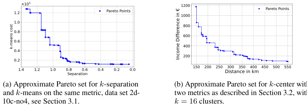
🔼 This figure shows two examples of approximate Pareto sets from the experimental sections of the paper. Subfigure (a) displays the trade-off between k-separation and k-means on the same metric, and subfigure (b) displays the trade-off between k-center with two different metrics. Each point in the plots represents a solution, and the area dominated by a solution lies to the right and above the corresponding point. The plots visually demonstrate the concept of the Pareto front, showing a set of solutions where there is no single solution that simultaneously optimizes both objectives. Each point in the Pareto set represents a good clustering that cannot be found by considering one of the objectives separately.
read the caption
Figure 3: Examples of approximate Pareto sets copied from the later experimental sections.

🔼 This figure visualizes the ground truth for three synthetic datasets used in the paper’s experiments. Each plot represents a different dataset (2d-4c-no3, 2d-10c-no3, 2d-10c-no4), showing the true cluster assignments for each data point. These visualizations help readers understand the underlying structure of the datasets and compare it against the clustering results produced by different algorithms.
read the caption
Figure 7: Visualization of the ground truth for the three synthetic data sets.

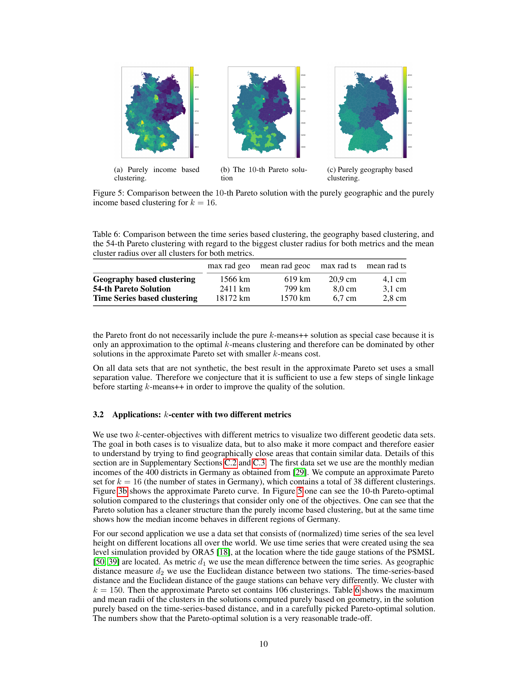
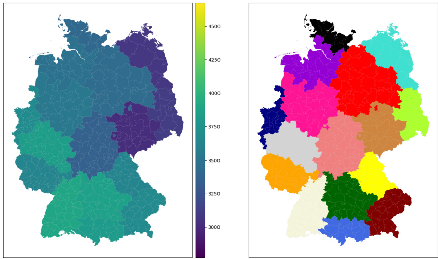
🔼 This figure compares three different clustering results for visualizing median incomes in Germany with k=16 clusters. (a) shows a clustering based solely on income, resulting in geographically dispersed clusters. (b) displays the 10th Pareto-optimal solution, which balances both geographic proximity and income similarity. Notice that this solution is more geographically coherent while still capturing the income structure. (c) presents a clustering focused only on geographic proximity, leading to clusters with a wide range of incomes.
read the caption
Figure 5. Comparison between the 10-th Pareto solution with the purely geographic and the purely income based clustering for k = 16.
🔼 This figure shows two examples of approximate Pareto sets. The first one shows the trade-off between k-separation and k-means on the same metric (use case 1), while the second one shows the trade-off between two k-center objectives with different metrics (use case 2). In both cases, the area dominated by a solution lies to the right and above the corresponding point. The approximate Pareto sets give a variety of trade-offs, offering more information and flexibility in data analysis.
read the caption
Figure 3: Examples of approximate Pareto sets copied from the later experimental sections.

🔼 This figure shows a simple example with four points on a line to illustrate the conflict between k-diameter and k-separation clustering objectives. The optimal k-diameter clustering (minimizing the maximum diameter of any cluster) results in a large distance between some points that are close together, while the optimal k-separation clustering (maximizing the minimum distance between clusters) may not be as good with respect to k-diameter. This highlights the need for finding Pareto-optimal solutions to address such trade-offs.
read the caption
Figure 1: A toy example.

🔼 This figure shows the ground truth for three synthetic datasets used in the paper’s experiments. Each subplot represents a different dataset: (a) 2d-4c-no3, (b) 2d-10c-no3, and (c) 2d-10c-no4. The points are colored according to their cluster assignment in the ground truth, providing a visual representation of the true cluster structure for each dataset. These datasets are used to evaluate the performance of the proposed multi-objective clustering algorithms.
read the caption
Figure 7: Visualization of the ground truth for the three synthetic data sets.

🔼 This figure shows three different clusterings of the same 2D dataset (2d-10c-no4) with 10 clusters. (a) shows the result of using the k-means++ algorithm. (b) shows the result of using Single Linkage clustering. (c) shows the best clustering found on the approximate Pareto curve. The Pareto curve in this case balances k-separation (maximizing the minimum distance between clusters) and k-means (minimizing the sum of squared distances to cluster centers). The figure illustrates the trade-off between these two often conflicting objectives. k-means++ produces a good clustering in terms of minimizing the sum of squared distances, but the clusters are not well-separated. Single linkage produces well-separated clusters, but at the cost of high squared distances to cluster centers. The Pareto-optimal solution provides a balanced compromise, achieving reasonably well-separated clusters with relatively low squared distances to cluster centers.
read the caption
Figure 4: Clusterings computed on data set 2d-10c-no4 by Handl and Knowles [33].
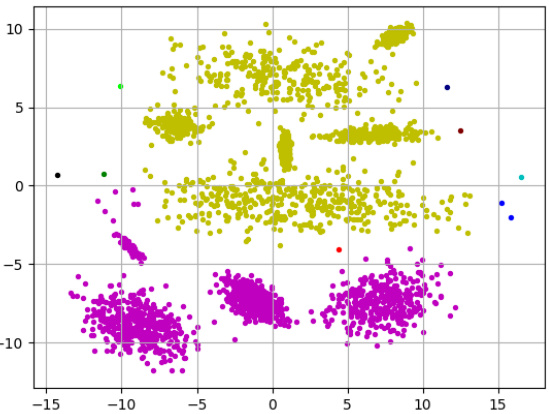
🔼 This figure visualizes the clustering results obtained using different methods on the 2d-10c-no4 dataset. It showcases three separate clusterings generated via three distinct methods: (a) k-means++, (b) Single Linkage, and (c) a solution selected from the approximate Pareto curve. This comparison aims to highlight the advantages and drawbacks of each method in terms of cluster shape, separation, and overall accuracy in capturing the underlying structure of the dataset.
read the caption
Figure 4: Clusterings computed on data set 2d-10c-no4 by Handl and Knowles [33].
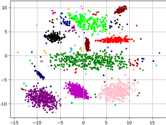
🔼 The figure shows three different clusterings of the same data set (2d-10c-no4) produced by three different methods: k-means++, Single Linkage, and the best clustering found on the approximate Pareto curve. The data set consists of points in a two-dimensional space, and the ground truth consists of 10 clusters. The k-means++ algorithm produces a clustering that is reasonably close to the ground truth, but some clusters are split or merged. The Single Linkage algorithm produces a very different clustering, that contains two large clusters and 8 small clusters, largely due to outliers. The best clustering on the approximate Pareto curve is much closer to the ground truth, and has a more balanced trade-off between different objectives than k-means++ or Single Linkage.
read the caption
Figure 4: Clusterings computed on data set 2d-10c-no4 by Handl and Knowles [33].

🔼 This figure shows three different clusterings of the same dataset (2d-10c-no4), each with 10 clusters. (a) shows a clustering generated using the k-means++ algorithm, (b) shows a clustering produced by Single Linkage, and (c) shows the best clustering found on the approximate Pareto curve, which represents a trade-off between multiple objectives. The visualization allows for a comparison of the three different approaches and their performance in terms of cluster separation and data homogeneity. The differences highlight the inherent conflict between various clustering objectives and the benefits of considering multiple objectives simultaneously to find a balanced solution.
read the caption
Figure 4: Clusterings computed on data set 2d-10c-no4 by Handl and Knowles [33].

🔼 This figure shows three different clusterings of the same dataset (2d-10c-no4) created by three different methods. (a) shows a clustering performed by the k-means++ algorithm, resulting in a clustering that mostly captures the ground truth but has some inaccuracies due to its limitations. (b) shows a clustering performed by Single Linkage, which is overly sensitive to outliers resulting in an inaccurate clustering. (c) shows a clustering that is chosen from the approximate Pareto set, achieving a better balance between the two objectives of accurate clustering and good separation.
read the caption
Figure 4: Clusterings computed on data set 2d-10c-no4 by Handl and Knowles [33].
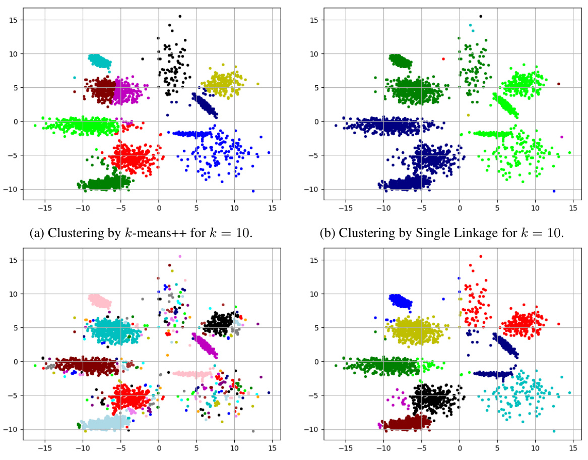
🔼 This figure shows three different clusterings of the same dataset (2d-10c-no4 from Handl and Knowles [33]), each with k=10 clusters. (a) shows a clustering produced by the k-means++ algorithm. (b) shows a clustering produced by the Single Linkage algorithm. (c) shows the best clustering found among the approximate Pareto set, demonstrating a combination of the strengths of k-means++ and Single Linkage, producing a superior clustering compared to the other two.
read the caption
Figure 4: Clusterings computed on data set 2d-10c-no4 by Handl and Knowles [33].
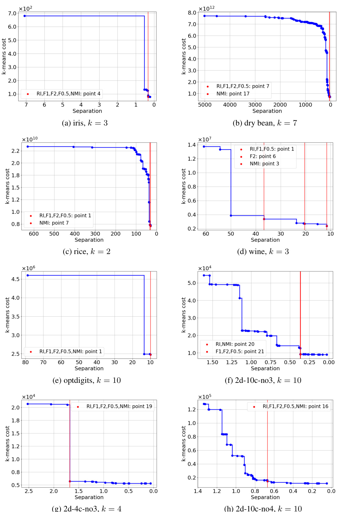
🔼 This figure shows two examples of approximate Pareto sets for bi-objective clustering problems. Subfigure (a) illustrates the trade-off between k-separation and k-means using the same metric (use case 1). Subfigure (b) displays the trade-off between two k-center objectives, but using different metrics derived from map design (use case 2). The area dominated by a given solution lies to the right and above its plotted point.
read the caption
Figure 3: Examples of approximate Pareto sets copied from the later experimental sections.
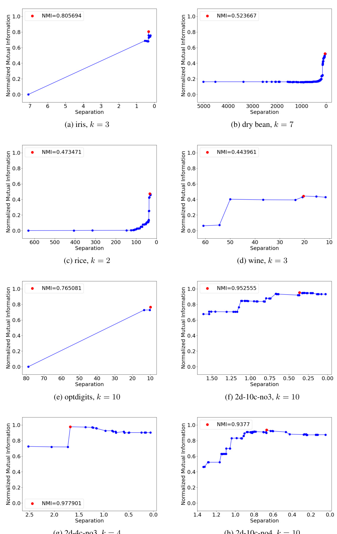
🔼 The figure contains two subfigures showing examples of approximate Pareto sets for different combinations of clustering objectives. Subfigure (a) shows the trade-off between k-separation and k-means on the same metric, while subfigure (b) shows the trade-off between two k-center objectives with two different metrics. The Pareto sets represent the set of non-dominated solutions, offering a range of trade-offs between the chosen objectives. These Pareto fronts provide insights into the different balancing points between conflicting objectives, such as achieving good cluster separation while also minimizing k-means cost or optimizing k-center under different distance metrics.
read the caption
Figure 3: Examples of approximate Pareto sets copied from the later experimental sections.
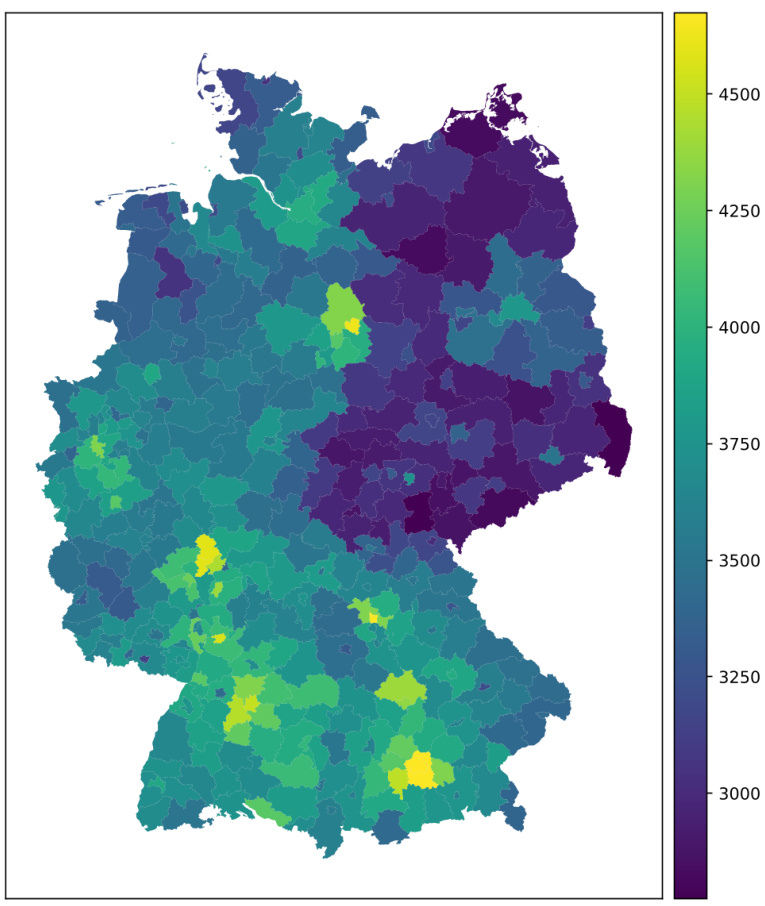
🔼 This figure shows a choropleth map of Germany, where each district is colored based on its median monthly income. The color scale ranges from dark purple (lowest income) to bright yellow (highest income), providing a visual representation of income distribution across the country. It illustrates regional income variations, with some areas showing significantly higher incomes compared to others. The map provides a clear overview of the income disparity within Germany, highlighting potential areas of economic inequality or focusing areas for economic policy consideration.
read the caption
Figure 15: Visualization of the median monthly incomes in Germany (in Euro).

🔼 This figure shows the Pareto curve obtained by applying the proposed multi-objective clustering algorithm for k=16. The x-axis represents the maximum geographic distance between any two points within a cluster (in kilometers), and the y-axis represents the maximum difference in median income (in Euros) between any two districts within a cluster. Each point on the curve represents a Pareto-optimal clustering solution, meaning there is no other solution that simultaneously improves both the geographic compactness and income homogeneity. The 10th and 15th solutions are highlighted with red squares, indicating specific clusterings that offer a particular trade-off between these two objectives. The shape of the curve itself shows the inherent conflict between these two objectives: improving one typically worsens the other.
read the caption
Figure 16: The resulting Pareto curve for k = 16. The 10-th and 15-th solution are marked with red squares.

🔼 This figure shows the Pareto curve obtained by the algorithm for the case k=16 (number of clusters). The x-axis represents the geographic distance in kilometers, and the y-axis represents the difference in median income (in Euros) between districts within the same cluster. The plot displays a set of non-dominated solutions (Pareto front), representing trade-offs between minimizing geographic spread and income disparity within clusters. The 10th and 15th solutions along the curve are highlighted with red squares, indicating particular trade-offs between spatial compactness and income homogeneity that might be of interest to the researchers.
read the caption
Figure 16. The resulting Pareto curve for k = 16. The 10-th and 15-th solution are marked with red squares.

🔼 This figure shows a comparison of three different clusterings of the 400 German districts based on their median income. (a) shows a purely income-based clustering, where districts are grouped solely by income similarity, regardless of geographic location. (b) depicts the 10th Pareto-optimal solution from a bi-objective optimization that considers both income similarity and geographic proximity. This solution represents a trade-off between the two objectives, aiming for clusters that are both income-homogeneous and geographically compact. (c) illustrates a purely geography-based clustering, focusing solely on geographic proximity. By comparing these three visuals, one can see how the Pareto-optimal solution finds a balance between income homogeneity and geographic compactness, offering a more informative clustering than either extreme approach.
read the caption
Figure 5: Comparison between the 10-th Pareto solution with the purely geographic and the purely income based clustering for k = 16.

🔼 This figure shows a choropleth map of Germany, where each district is colored according to its median monthly income. The color scale represents the income levels, ranging from approximately 3000 Euros to over 4500 Euros. The map provides a visual representation of income distribution across different regions of Germany, highlighting areas of higher and lower average income.
read the caption
Figure 15: Visualization of the median monthly incomes in Germany (in Euro).
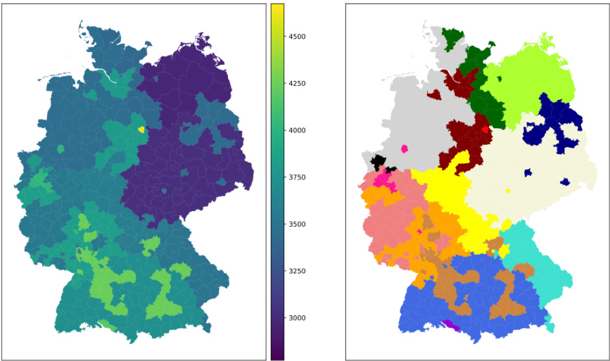
🔼 This figure compares three different clustering results for k=16: one that only considers income (left), one that only considers geographic distance (right), and the 10th solution from the approximate Pareto set (middle). The differences illustrate the tradeoff between the two objectives. The Pareto solution aims to achieve a balance by presenting a compromise between income homogeneity and geographical proximity.
read the caption
Figure 18. Comparison between the 10-th Pareto solution with the purely geographic and the purely income based clustering for k = 16.
🔼 This figure shows a choropleth map of Germany, where each district is colored according to its median monthly income in Euros. The color scale ranges from approximately 3000 Euros to 4500 Euros, illustrating the income distribution across the country. Darker colors represent higher incomes, while lighter colors represent lower incomes. The map provides a visual representation of regional income disparities within Germany.
read the caption
Figure 15: Visualization of the median monthly incomes in Germany (in Euro).
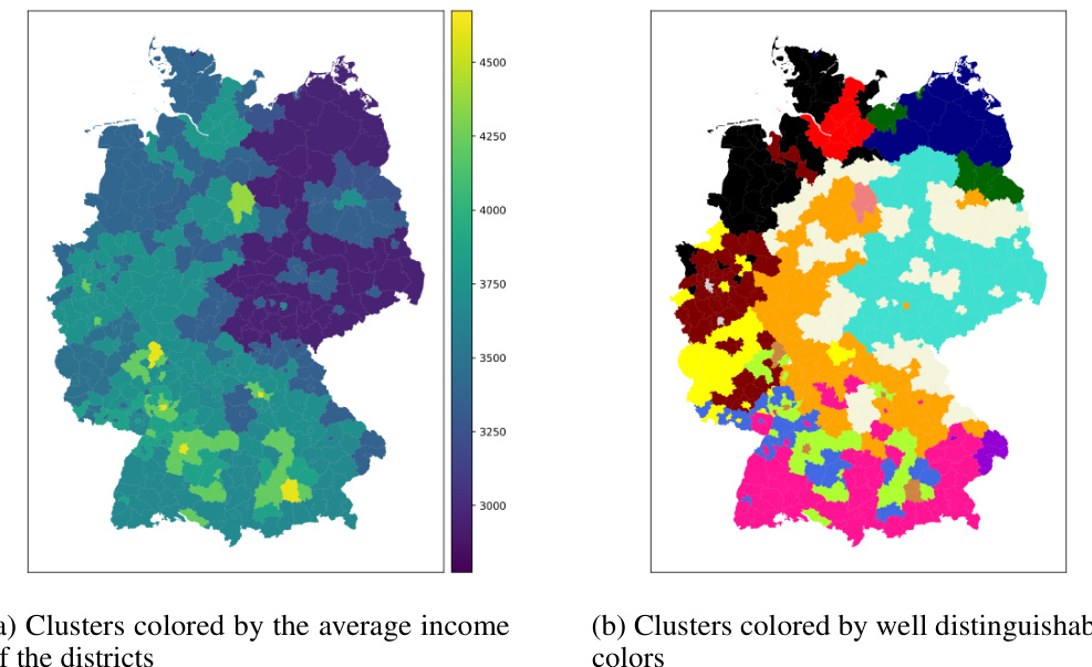
🔼 This figure compares three different clusterings of German districts based on median income and geographic location. The leftmost image shows a clustering based solely on income, resulting in geographically dispersed clusters. The rightmost image shows a clustering based solely on geographic proximity, leading to clusters with a wide range of income levels. The center image depicts the 10th solution from the approximate Pareto set, which represents a trade-off between income homogeneity and geographic compactness. This solution aims to find clusters that are both geographically coherent and relatively homogenous in terms of income. The visualization clearly shows how the Pareto-optimal solution balances the two objectives, offering a compromise between the other two solutions that offers more insights.
read the caption
Figure 19: Comparison between the 10-th Pareto solution with the purely geographic and the purely income-based clustering for k = 16. The clusters are once colored according to the average income over all districts in that cluster (left) and once with well distinguishable colors (right).
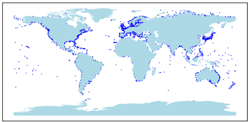
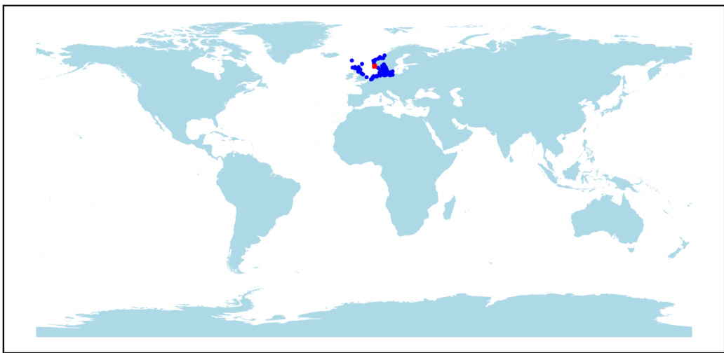
🔼 This figure shows the geographic locations of 1581 tide gauge stations around the world, most situated along coastlines. These stations measure sea levels, providing data for the study’s time-series analysis. The distribution of stations is not uniform globally, with higher concentrations in certain areas.
read the caption
Figure 21: Positions of the PSMSL tide gauge stations.
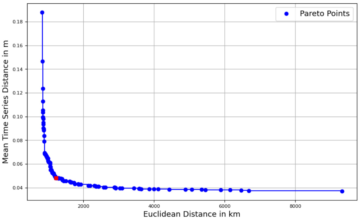
🔼 This figure shows the approximate Pareto curve obtained for clustering sea level data using two k-center objectives (geographic distance and mean time series distance) with k=150 clusters. The x-axis represents the Euclidean distance (in km) between cluster centers, while the y-axis represents the mean time series distance (in m) between time series within the same cluster. The curve illustrates the trade-off between these two objectives. The point highlighted in red corresponds to the 54th solution on the Pareto front, representing a compromise between geographic compactness and similarity of time series within clusters.
read the caption
Figure 22: Approximate Pareto curve for the sea level data for k=150. The 54-th approximate Pareto solution is highlighted in red.

🔼 This figure shows the geographical locations of 1581 tide gauge stations from the Permanent Service for Mean Sea Level (PSMSL) dataset. These stations are located around the world, predominantly along coastlines, and record monthly sea level data. The map provides a visual representation of the global distribution of these stations, highlighting their concentration in certain regions (e.g., Europe, North America) while showing a relative scarcity in others. This distribution is relevant to the study’s analysis of clustering these stations based on both their geographical proximity and the similarity of their recorded time series.
read the caption
Figure 21: Positions of the PSMSL tide gauge stations.

🔼 This figure shows the geographical locations of 1581 tide gauge stations around the world. These stations are part of the Permanent Service for Mean Sea Level (PSMSL) dataset and measure sea level at their respective locations. The map displays the distribution of these stations across various coastlines and oceans. The concentration of stations in the Northern Hemisphere is higher than in the Southern Hemisphere.
read the caption
Figure 21: Positions of the PSMSL tide gauge stations.
🔼 This figure shows the geographical locations of the 1581 tide gauge stations used in the sea level data clustering experiments. The stations are spread across the globe, but with a higher concentration in the Northern Hemisphere and along coastlines.
read the caption
Figure 21: Positions of the PSMSL tide gauge stations.
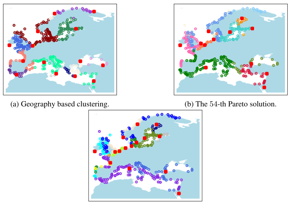
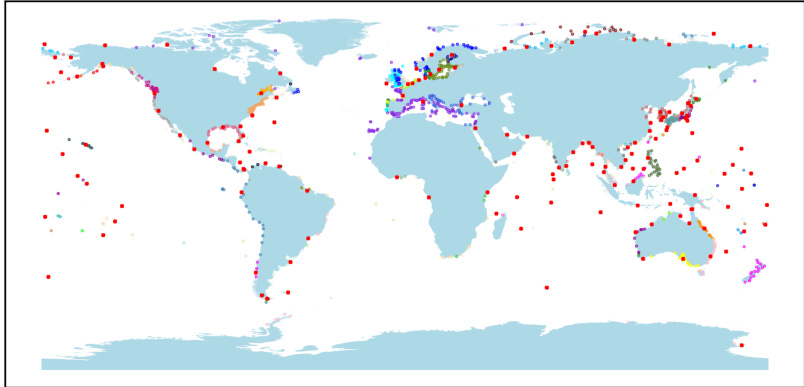
🔼 This figure compares three different clustering approaches applied to the European region of the sea level data. The top panel shows the geographically-based clustering which focuses on grouping geographically close stations. The middle panel presents the 54th solution from the approximate Pareto front, which balances geographic proximity with time series similarity. The bottom panel displays the time-series-based clustering, focusing solely on the similarity of sea level patterns over time. The red squares indicate the cluster centers in each clustering.
read the caption
Figure 24. The geography based clustering, the 54-th Pareto solution, and the time series based clustering in the area of Europe. Centers are drawn in red.

🔼 This figure visualizes the clustering results on the 2d-10c-no4 dataset using three different methods: k-means++, single linkage, and the best clustering from the approximate Pareto curve. (a) shows the k-means++ clustering, illustrating how some clusters are split or merged due to the algorithm’s limitations. (b) demonstrates the single linkage clustering, where most points are merged into two large clusters. (c) presents the single linkage clustering obtained with a specific separation value (0.67), revealing a better separation of clusters but with a larger number of clusters than in (a) or (b). Finally, (d) displays the best clustering found in the approximate Pareto set (a trade-off between k-separation and k-means++), successfully finding the important clusters while maintaining a balance of cluster separation and the number of clusters.
read the caption
Figure 8: Clusterings computed on data set 2d-10c-no4.
🔼 This figure shows the ground truth visualization of three synthetic datasets used in the paper’s experiments. Each dataset represents a different clustering scenario, with varying levels of cluster separation and complexity. Visualizing the ground truth helps in evaluating the performance of clustering algorithms by comparing the produced clusters to the actual structure present in the data.
read the caption
Figure 7: Visualization of the ground truth for the three synthetic data sets.

🔼 This figure visualizes the ground truth for three synthetic datasets used in the paper’s experiments. Each dataset represents a 2D point set with a certain number of clusters. The visualization helps to understand the structure of the data and evaluate the performance of the proposed clustering algorithms against a known ideal outcome.
read the caption
Figure 7: Visualization of the ground truth for the three synthetic data sets.

🔼 This figure shows the geographical locations of 1581 tide gauge stations around the world, which are part of the Permanent Service for Mean Sea Level (PSMSL) dataset. The data from these stations is used in the paper to perform a clustering analysis of sea level behavior. The concentration of stations is not even across the globe, with a higher concentration in the northern hemisphere, particularly along coastlines.
read the caption
Figure 21: Positions of the PSMSL tide gauge stations.
More on tables

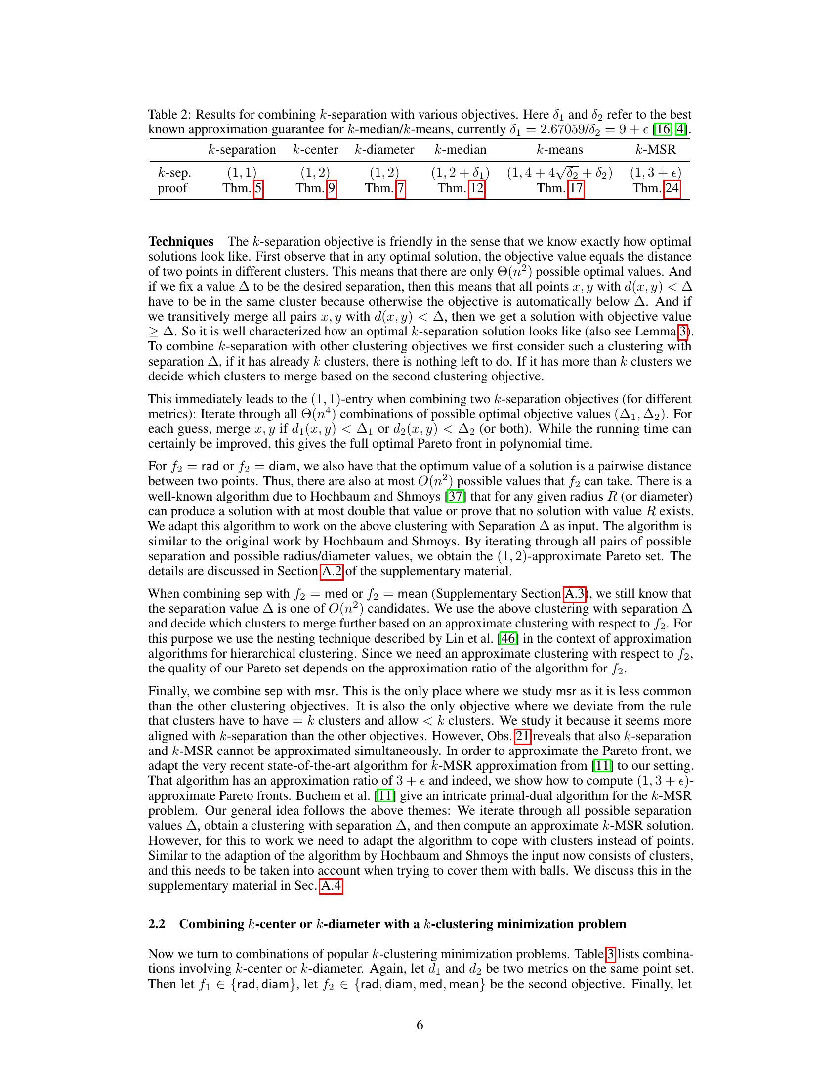
🔼 This table presents the approximation factors achieved by the algorithms developed in the paper for computing approximate Pareto sets when combining the k-separation objective with various other k-clustering minimization objectives (k-center, k-diameter, k-median, k-means, k-MSR). The approximation factors are given as pairs (α₁, α₂), where α₁ refers to the approximation factor for k-separation and α₂ refers to the approximation factor for the second objective. The table also notes that δ₁ and δ₂ represent the best-known approximation guarantees for k-median and k-means, respectively.
read the caption
Table 2: Results for combining k-separation with various objectives. Here δ₁ and δ₂ refer to the best known approximation guarantee for k-median/k-means, currently δ₁ = 2.67059/δ₂ = 9 + є [16, 4].

🔼 This table presents approximation factors achieved by the authors’ algorithms when combining k-center or k-diameter objectives with k-median or k-means objectives. The approximation factor is represented as a pair (a, b), where ‘a’ is the approximation factor for the first objective (k-center or k-diameter), and ‘b’ is the approximation factor for the second objective (k-median or k-means). The table indicates that the algorithms achieve different approximation guarantees depending on the specific combination of objectives and whether different metrics are used for each objective. It also notes that results for combining k-center/k-diameter with k-separation are detailed in a different table.
read the caption
Table 3: Results for combining rad and diam for two different metrics or with a sum-based objective. The combination of k-center/k-diameter with k-separation can be found in Table 2.

🔼 This table presents approximation guarantees for combining k-separation with other k-clustering objectives. It shows the approximation factors achieved for the Pareto set using different combinations of two objectives (k-separation paired with k-center, k-diameter, k-median, k-means, and k-MSR). The table indicates the approximation factors (a1, a2) obtained, where a1 refers to the k-separation approximation and a2 indicates the approximation for the second objective. The ‘proof’ column references the theorem in the supplementary material which proves the approximation guarantee.
read the caption
Table 2: Results for combining k-separation with various objectives. Here δ₁ and δ₂ refer to the best known approximation guarantee for k-median/k-means, currently δ₁ = 2.67059/δ₂ = 9 + є [16, 4].

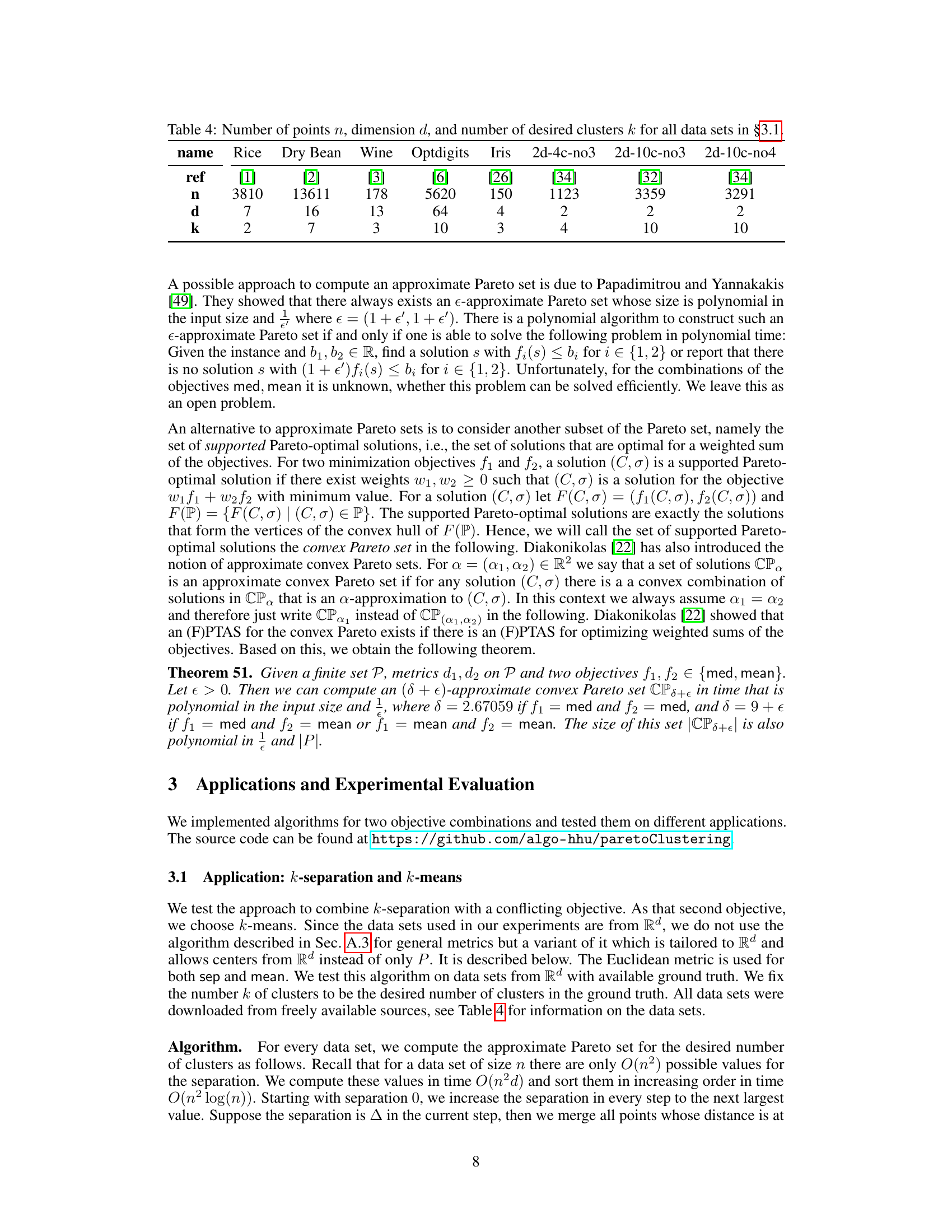
🔼 This table presents the results of comparing three different clustering methods on several datasets. The Normalized Mutual Information (NMI) score is used to measure the quality of the clustering results, which indicates how well the generated clusters correspond to the ground truth clusters. The three methods compared are: 1. Single Linkage (SL): A hierarchical clustering method. 2. k-means++ (kM++): A well-known partitional clustering method. 3. Best solution from the Pareto Set (C):* The best clustering solution obtained using the proposed multi-objective approach, which optimizes both cluster separation and k-means simultaneously. The table shows the average NMI scores obtained for each method over 20 independent runs for each dataset. This allows a comparison of clustering performance to identify which method produces the best results on each dataset.
read the caption
Table 5: NMI of the best solutions by single linkage and k-means++, and of the best solution C* in the Pareto set. Randomized algorithms were repeated 20 times and values are then averages.

🔼 This table summarizes the approximation factors achieved by the proposed algorithms for approximating the Pareto front when combining k-separation with other k-clustering objectives (k-center, k-diameter, k-median, k-means, k-MSR). The approximation factors are given as pairs (α₁, α₂), where α₁ refers to the approximation factor for k-separation and α₂ for the second objective. The table also indicates the theorem in the supplementary material where each result is proved. The table highlights the trade-offs and challenges in approximating different combinations of objectives. The values of δ₁ and δ₂ are the approximation guarantees for k-median and k-means respectively, taken from existing literature.
read the caption
Table 2: Results for combining k-separation with various objectives. Here δ₁ and δ₂ refer to the best known approximation guarantee for k-median/k-means, currently δ₁ = 2.67059/δ₂ = 9 + є [16, 4].

🔼 This table presents the approximation guarantees achieved by the algorithms for computing approximate Pareto sets when combining the k-separation objective with various other k-clustering minimization objectives (k-center, k-diameter, k-median, k-means, and k-MSR). The approximation factors are given as pairs (α₁, α₂), indicating that the algorithm provides a solution within a factor of α₁ of the optimal k-separation solution and within a factor of α₂ of the optimal solution for the second objective. The table also indicates the theorems in supplementary material that provide proofs for the approximation guarantees.
read the caption
Table 2: Results for combining k-separation with various objectives. Here δ₁ and δ₂ refer to the best known approximation guarantee for k-median/k-means, currently δ₁ = 2.67059/δ₂ = 9 + є [16, 4].

🔼 This table presents the approximation factors achieved by the algorithms developed in the paper for computing approximate Pareto sets when combining the k-separation objective with various other k-clustering minimization objectives (k-center, k-diameter, k-median, k-means, k-MSR). The approximation factors (a1, a2) indicate that the algorithms guarantee that for every Pareto-optimal solution, there exists a solution in the approximate Pareto set within a factor of a1 for the k-separation objective and a2 for the secondary objective.
read the caption
Table 2: Results for combining k-separation with various objectives. Here δ₁ and δ₂ refer to the best known approximation guarantee for k-median/k-means, currently δ₁ = 2.67059/δ₂ = 9 + ε [16, 4].

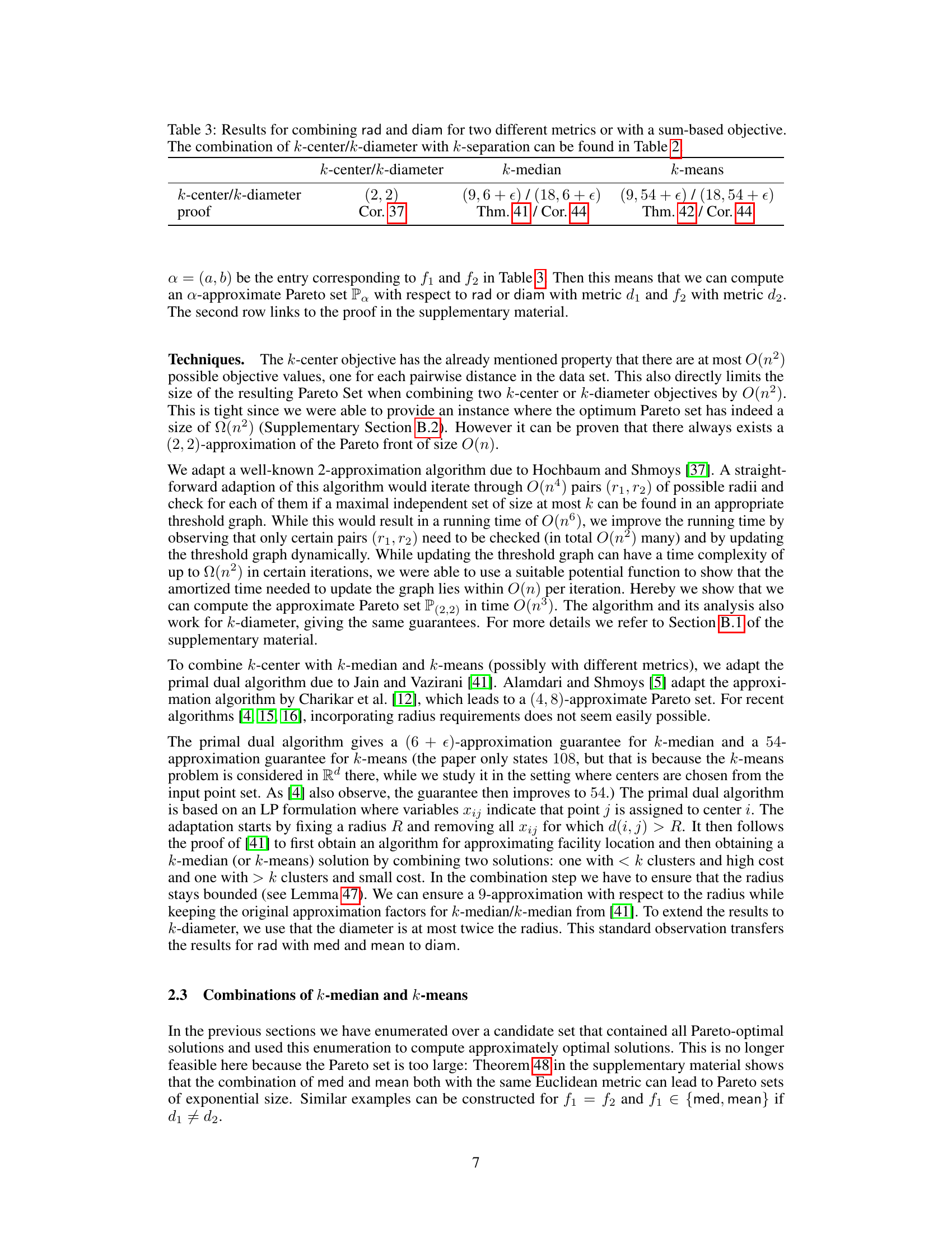
🔼 This table presents approximation factors achieved by the algorithms for approximating Pareto fronts for various combinations of k-separation with other k-clustering objectives (k-center, k-diameter, k-median, k-means, k-MSR). The approximation guarantee is given as a pair (a, b), where a is the approximation factor for k-separation, and b is the approximation factor for the second objective. The table shows that the developed algorithms achieve provable approximation guarantees. For example, the (1, 2) approximation for k-center/k-diameter indicates that the resulting approximate Pareto set provides a 1-approximation for k-separation and a 2-approximation for k-diameter.
read the caption
Table 2: Results for combining k-separation with various objectives. Here δ₁ and δ₂ refer to the best known approximation guarantee for k-median/k-means, currently δ₁ = 2.67059/δ₂ = 9 + є [16, 4].
Full paper#
