TL;DR#
Many real-world systems exhibit causal interactions best described by mixtures of Directed Acyclic Graphs (DAGs), rather than single DAGs. Existing methods struggle with inherent uncertainty regarding the component DAG structures, and potentially cyclic relationships between components. This makes identifying the true causal relationships (i.e., edges present in at least one component DAG) a significantly harder problem.
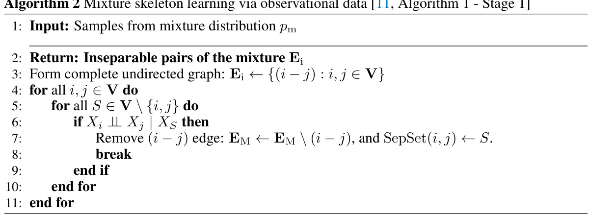
This paper addresses these challenges by proposing a novel algorithm, CADIM, which uses interventions to learn these true causal edges. It provides both necessary and sufficient conditions for the intervention sizes needed to reliably learn these edges. The algorithm’s efficiency is analyzed, revealing a performance gap tied to the cyclic complexity of the mixture. The results offer important theoretical insights and practical tools for causal discovery in complex systems.
Key Takeaways#
Why does it matter?#
This paper is crucial for researchers in causal inference and related fields because it tackles the challenging problem of causal discovery in complex systems that cannot be represented by a single causal graph. The proposed adaptive algorithm, with its optimality guarantees and efficient intervention design, paves the way for more accurate and reliable causal analysis in diverse applications, from genomics to dynamical systems. Its findings also provide theoretical insights into the limitations and potential of interventions in causal discovery, which is relevant to researchers working on both observational and experimental designs.
Visual Insights#

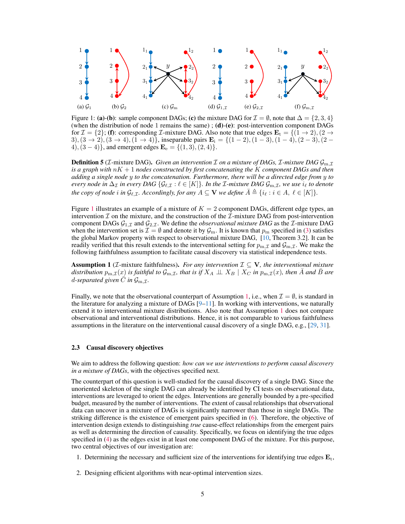
🔼 This figure shows an example with two component DAGs, G1 and G2. The mixture DAG Gm (c) illustrates the combined structure without intervention. The post-intervention DAGs G1,I and G2,I (d, e) are shown after intervening on node 2 (I={2}). Finally, Gm,I (f) depicts the I-mixture DAG resulting from the intervention. The figure also highlights the true edges (Et), inseparable pairs (Ei), and emergent edges (E) illustrating the challenges of causal discovery in mixtures of DAGs.
read the caption
Figure 1: (a)-(b): sample component DAGs; (c) the mixture DAG for I = Ø, note that ∆ = {2,3,4} (when the distribution of node 1 remains the same) ; (d)-(e): post-intervention component DAGs for I = {2}; (f): corresponding I-mixture DAG. Also note that true edges Et = {(1 → 2), (2 → 3), (3 → 2), (3 → 4), (1 → 4)}, inseparable pairs E₁ = {(1 − 2), (1 – 3), (1 – 4), (2 – 3), (2 – 4), (3-4)}, and emergent edges E = {(1, 3), (2, 4)}.
In-depth insights#
Mixture DAGs#
The concept of “Mixture DAGs” introduces a significant advancement in causal discovery by moving beyond the limitations of single DAG models. It acknowledges the complexity of real-world systems, where multiple causal mechanisms might coexist and interact. This approach uses a mixture of multiple DAGs to represent the system, capturing the nuances of different causal structures that may operate concurrently or under specific conditions. The challenge lies in disentangling these overlapping DAGs and identifying the true causal relationships. Addressing the inherent uncertainty about the skeletons and the potential for cyclic relationships across the component DAGs are crucial steps in the development of robust algorithms for causal discovery. This approach brings a more realistic and flexible framework, though it poses considerable algorithmic and computational challenges, requiring innovative solutions to handle the increased complexity. The work on intervention design for Mixture DAGs is particularly promising, suggesting a potential path toward resolving identifiability issues and achieving more accurate causal inference.
Intervention Size#
The heading ‘Intervention Size’ likely explores the minimum number of variables that need to be manipulated during interventions to effectively learn causal relationships from a mixture of directed acyclic graphs (DAGs). The authors likely investigate the trade-off between intervention complexity and the identifiability of true causal edges. Sufficient conditions for intervention size likely involve establishing a lower bound on the number of variables needed to break certain dependencies, while necessary conditions might focus on the minimal intervention size to distinguish true edges from spurious associations. The analysis likely includes scenarios with varying causal structures and cyclic complexities within the DAG mixture, showing how optimal intervention size might change depending on the complexity of the underlying causal system. The paper likely derives both theoretical bounds and algorithm-specific analyses of the intervention sizes, demonstrating the potential optimality of proposed algorithms under specific conditions. Optimal intervention size is probably discussed for both general DAG mixtures and simpler cases like mixtures of trees, and possibly highlights situations where near-optimal intervention sizes might be sufficient, or the gap between the algorithmic and optimal sizes could be quantified.
Adaptive Algorithm#
An adaptive algorithm, in the context of interventional causal discovery within a mixture of DAGs, is crucial for efficiently identifying true causal relationships. The algorithm’s adaptive nature is key because the optimal intervention size varies depending on the underlying causal structure. The algorithm intelligently adjusts the size and number of interventions based on the observed data, dynamically responding to the complexity of the mixture model. This adaptive approach helps to minimize the total number of interventions required, thereby enhancing efficiency and reducing experimental costs. The algorithm’s optimality is particularly notable in cases where the mixture DAGs are cycle-free, demonstrating significant efficiency gains compared to non-adaptive methods. However, even in scenarios with cyclic dependencies across component DAGs, the gap between the algorithm’s intervention size and the optimal size remains bounded, offering a quantifiable measure of suboptimality. This makes the adaptive algorithm highly valuable for real-world applications where complete a priori knowledge about the causal structure may be unavailable. The algorithm’s performance hinges on the accuracy of conditional independence (CI) tests used within the algorithm, highlighting a potential avenue for further improvement.**
Optimality Gap#
The optimality gap in the context of interventional causal discovery in a mixture of DAGs refers to the difference between the maximum intervention size used by an algorithm and the optimal intervention size. This gap arises because algorithms must handle the complexities of cyclic relationships across component DAGs, unlike the simpler case of single DAGs. The authors quantify this gap using the concept of cyclic complexity, which represents the minimum size of an intervention needed to break cycles among the ancestors of a node. A key insight is that the gap is bounded by the cyclic complexity, implying that for acyclic mixtures, the algorithms achieve the optimal intervention size. However, for cyclic mixtures, the algorithms may require interventions larger than the theoretical minimum, although the gap remains quantifiable and manageable.
Future Research#
Future research directions stemming from this work on interventional causal discovery in mixture DAGs could explore several promising avenues. Relaxing assumptions about the underlying data generating process, such as the faithfulness assumption or the nature of the intervention, would enhance the applicability and robustness of the methods. Investigating the impact of latent variables and developing techniques to handle them effectively is crucial. Extending the algorithmic framework to incorporate different types of interventions or handle larger-scale problems more efficiently is another key area. Finally, exploring the potential for practical applications in various fields, and rigorously validating the approach on real-world datasets, will further solidify its impact and usefulness. Theoretical advancements could focus on establishing tighter bounds on intervention sizes and further characterizing the relationships between intervention strength, identifiability, and the structure of the component DAGs. The research could also be advanced by developing methods capable of automatically learning the number of component DAGs involved in a mixture model.
More visual insights#
More on figures

🔼 This figure presents the results of experiments evaluating the performance of the proposed algorithm. Subfigure (a) compares the true edge recovery rate of the algorithm with an observation-based approach, demonstrating the advantage of the interventional method. Subfigure (b) illustrates the algorithm’s scalability by showing that the true edge recovery rate remains consistently high even as the number of nodes increases. Finally, subfigure (c) quantifies the empirical cyclic complexity for varying numbers of nodes and mixture components (K), showing that this complexity remains relatively low, even for larger mixtures, which impacts the algorithm’s optimality.
read the caption
Figure 2: Mean true edge recovery rates and quantification of mean cyclic complexity of a node.

🔼 This figure shows an example with two component DAGs (G1 and G2). Part (c) displays the mixture DAG (Gm) resulting from combining G1 and G2, highlighting the set ∆ of nodes with different conditional distributions across the DAGs. Parts (d) and (e) illustrate the post-intervention component DAGs (G1,I and G2,I) after performing an intervention on node 2 (I = {2}). Finally, part (f) shows the resulting I-mixture DAG (Gm,I), which incorporates the intervention’s effect. The caption also labels the true edges (Et), inseparable pairs (Eᵢ), and emergent edges (E).
read the caption
Figure 1: (a)-(b): sample component DAGs; (c) the mixture DAG for I = Ø, note that ∆ = {2,3,4} (when the distribution of node 1 remains the same) ; (d)-(e): post-intervention component DAGs for I = {2}; (f): corresponding I-mixture DAG. Also note that true edges Et = {(1 → 2), (2 → 3), (3 → 2), (3 → 4), (1 → 4)}, inseparable pairs Eᵢ = {(1 − 2), (1 – 3), (1 – 4), (2 – 3), (2 – 4), (3-4)}, and emergent edges E = {(1, 3), (2, 4)}.
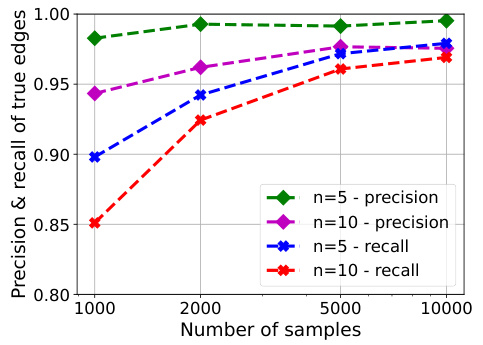
🔼 Figure 4 shows the performance of Algorithm 1 on the task of recovering true edges under varying numbers of samples and graph sizes. The plots show that the algorithm achieves almost perfect precision even with relatively small sample sizes. The recall rates are lower than the precision initially, but improve and approach the precision as the number of samples increases.
read the caption
Figure 4: Additional experiment results for true edge recovery

🔼 This figure presents the results of experiments evaluating the performance of the CADIM algorithm. Subfigure (a) compares the true edge recovery rates of the proposed interventional approach with the performance of an observational-only method, demonstrating the advantage of using interventions. Subfigure (b) shows that the algorithm maintains strong performance as the number of nodes in the network increases. Subfigure (c) presents the empirical cyclic complexity for different network sizes and numbers of component DAGs, showing that the complexity remains relatively low even for larger networks.
read the caption
Figure 2: Mean true edge recovery rates and quantification of mean cyclic complexity of a node.
🔼 This figure shows an example of a mixture of two DAGs (G1 and G2), illustrating the concepts of true edges, inseparable pairs, and emergent edges. It also demonstrates the construction of the I-mixture DAG from post-intervention component DAGs, showing how interventions can help to identify true causal relationships in a mixture of DAGs.
read the caption
Figure 1: (a)-(b): sample component DAGs; (c) the mixture DAG for I = Ø, note that ∆ = {2,3,4} (when the distribution of node 1 remains the same); (d)-(e): post-intervention component DAGs for I = {2}; (f): corresponding I-mixture DAG. Also note that true edges Et = {(1 → 2), (2 → 3), (3 → 2), (3 → 4), (1 → 4)}, inseparable pairs E₁ = {(1 − 2), (1 – 3), (1 – 4), (2 – 3), (2 – 4), (3-4)}, and emergent edges E = {(1, 3), (2, 4)}.
Full paper#

