TL;DR#
The field of machine learning faces challenges due to data scarcity. Many algorithms aim to improve sample efficiency, but lack theoretical guarantees. This paper introduces a new unifying concept, reciprocal learning, that encompasses various algorithms. These algorithms not only learn from data but also iteratively refine the data itself based on the model’s fit. This dynamic interaction addresses data limitations.
This paper presents a principled analysis of reciprocal learning using decision theory. It identifies conditions (non-greedy, probabilistic, and either randomized or regularized sample adaptation) under which reciprocal learning algorithms converge at linear rates. The authors prove convergence and offer insights into the relationship between the data and parameters. They extend their findings to established algorithms like self-training and active learning.
Key Takeaways#
Why does it matter?#
This paper is crucial for researchers in machine learning due to its introduction of the novel concept of reciprocal learning which provides a unifying framework for various algorithms that iteratively alter training data based on model fit. This offers new theoretical guarantees and insights into convergence, opening up avenues for designing efficient and reliable algorithms. It directly addresses the growing concerns over data scarcity in machine learning by promoting sample efficiency.
Visual Insights#
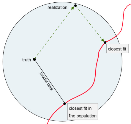
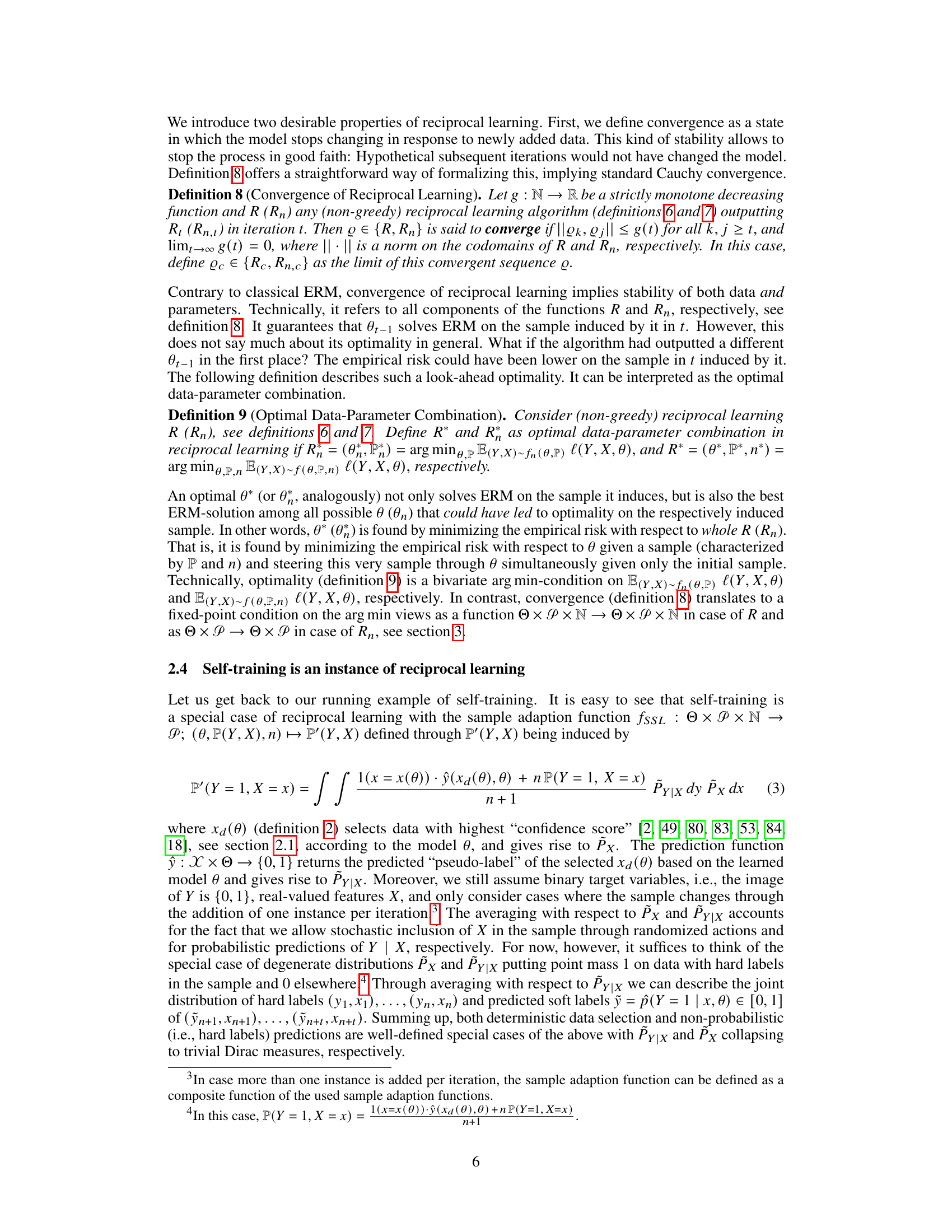
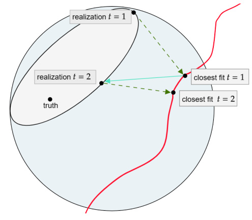
🔼 This figure illustrates the difference between classical machine learning and reciprocal learning. Panel (a) shows classical machine learning where the model is fitted to a static sample. Panel (b) shows reciprocal learning where the sample is iteratively altered based on the current model fit, creating a feedback loop between the model and data.
read the caption
Figure 1: (A) Classical machine learning fits a model from the model space (restricted by red curve) to a realized sample from the sample space (blue-grey); figure replicated from 'The Elements of Statistical Learning' [31, Figure 7.2]. (B) In reciprocal learning, the realized sample is no longer static, but changes in response to the model fit. Grey ellipse indicates restriction of sample space in t = 2 through realization in t = 1. Sample in t thus depends on model in t – 1 and sample in t−1.
In-depth insights#
Reciprocal Learning#
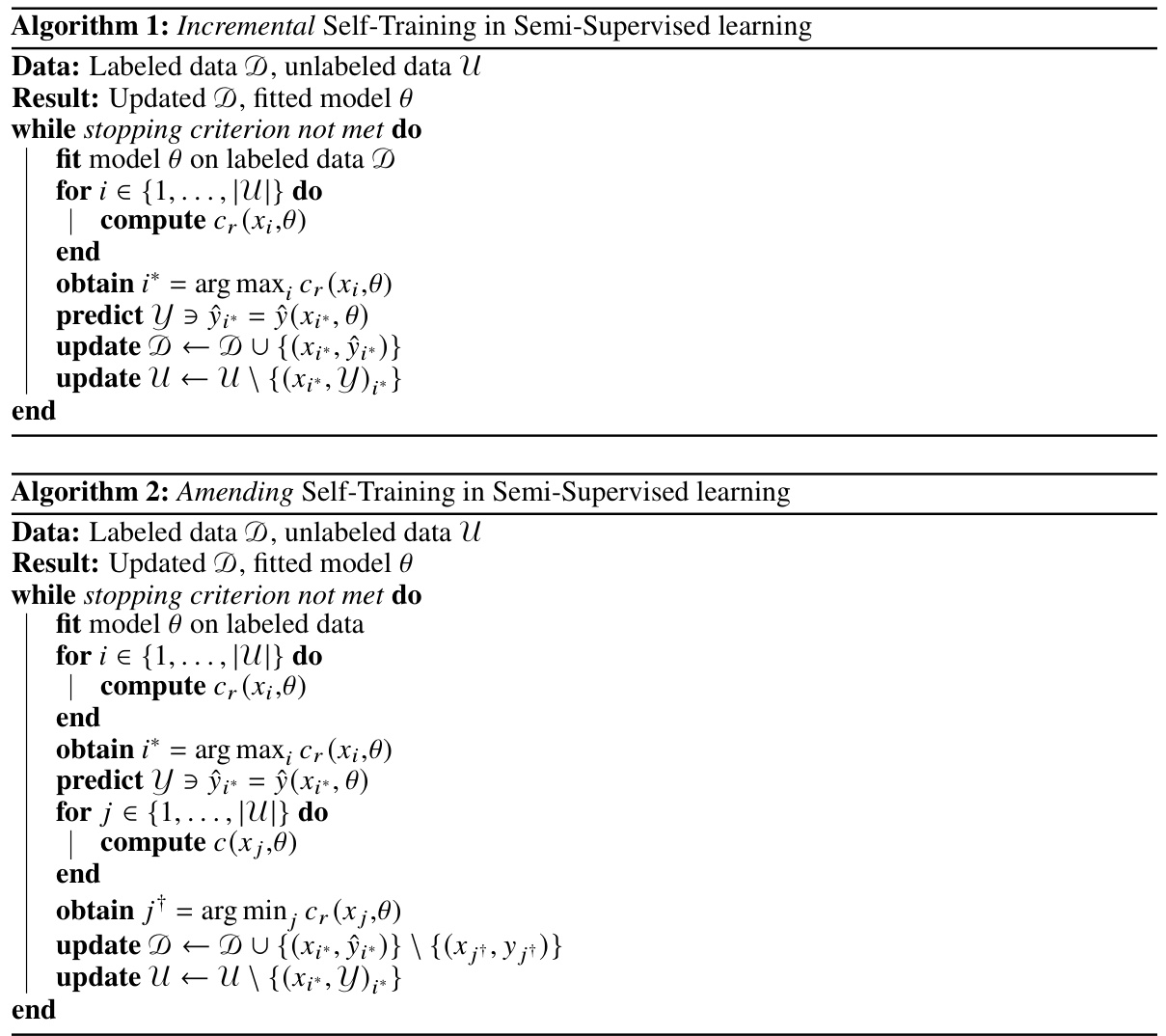
The concept of “Reciprocal Learning” introduces a novel paradigm in machine learning, shifting from the traditional unidirectional flow of information (data to parameters) to a bidirectional interaction. This reciprocal relationship, where the model’s current state influences the selection and modification of training data, is shown to unify various established algorithms like self-training, active learning, and multi-armed bandits. The core idea is iterative model fitting coupled with sample adaptation, a process that modifies the training data based on the model’s predictions or other criteria. The authors propose a theoretical framework to analyze convergence and optimality of such algorithms, identifying key conditions such as non-greedy data selection, probabilistic predictions, and regularization or randomization to ensure convergence at linear rates. This theoretical contribution provides a much-needed principled understanding of sample efficiency in these commonly used techniques and opens up new avenues for algorithm design and analysis.
Convergence Proofs#
Convergence proofs in machine learning rigorously establish that a learning algorithm will reach a stable solution given certain conditions. Central to these proofs is the demonstration of a contraction mapping, meaning that the algorithm’s iterative steps consistently reduce the distance to a fixed point, the optimal model. The Banach fixed-point theorem often underpins these arguments. Assumptions made are critical; common ones involve characteristics of the loss function (e.g., smoothness, convexity), the data distribution, and the algorithm’s update rule. A key consideration is demonstrating that the algorithm’s updates are Lipschitz continuous, implying a bounded change in output for a given change in input. The Lipschitz constant plays a crucial role, dictating the rate of convergence (linear in many cases) and influencing conditions for convergence. Finally, the type of data selection strategy (greedy vs. non-greedy) significantly affects the complexity of the convergence proof. Non-greedy strategies, which add and remove data, often require more sophisticated techniques to bound iterative changes, whereas greedy approaches can be comparatively simpler.
Algorithm Analysis#
A thorough algorithm analysis would dissect the paper’s methods, examining their time and space complexity, proving correctness, and establishing convergence rates. For machine learning algorithms, this might involve analyzing training time, prediction speed, and the algorithm’s ability to generalize to unseen data. Empirical validation through experiments on various datasets would be crucial, showcasing the algorithm’s performance in different settings and against other state-of-the-art methods. Statistical significance testing would ensure results are not due to chance. Furthermore, a robust analysis would explore the algorithm’s sensitivity to hyperparameters, providing guidance for optimal configuration, and address its scalability to handle larger datasets and more complex problems. The analysis should also discuss the algorithm’s limitations, outlining scenarios where it might underperform or fail completely, thereby providing a well-rounded evaluation of its practical utility.
Data Regularization#
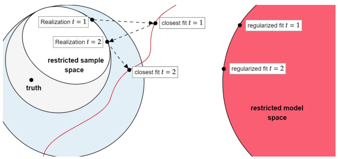
Data regularization, in the context of machine learning, is a crucial technique to enhance the stability and generalization ability of models. It involves modifying the data selection process to mitigate the impact of noise or outliers on model training. Unlike traditional regularization methods that focus on model parameters, data regularization directly addresses the quality and representativeness of the training data itself. This is particularly important in scenarios with limited, noisy, or biased data, which are increasingly common in real-world applications. The concept involves strategically selecting data points by adding a regularization term to the data selection criterion, which may incorporate techniques like adding randomness or constraints to ensure a balance between exploration and exploitation. This method leverages the idea that carefully chosen subsets of data can significantly improve model performance, thus aiming for optimal data-parameter combinations. The core idea is to constrain the data space to prevent overfitting. The effectiveness of data regularization is closely tied to the choice of regularization techniques and parameters – which must be carefully tuned according to the problem and dataset characteristics. A key advantage is its symmetry with parameter regularization, creating a balanced approach to improve model stability and generalization. Ultimately, data regularization offers a powerful tool for crafting more robust machine learning models that can generalize better to unseen data.
Future Research#
The ‘Future Research’ section of this hypothetical paper could explore several promising avenues. Extending the theoretical framework to encompass more complex scenarios, such as non-binary classification problems or settings with noisy labels, would be crucial. Investigating the impact of different regularization techniques on convergence and generalization performance warrants further investigation. A comprehensive empirical evaluation across diverse datasets and real-world applications would provide stronger evidence for the algorithm’s efficacy and robustness. Furthermore, developing more efficient algorithms that reduce computational complexity would increase its practical applicability. Finally, exploring the potential of combining reciprocal learning with other techniques, like transfer learning or meta-learning, could lead to innovative approaches with enhanced performance and data efficiency. These future studies would contribute significantly to advancing the understanding and applications of this promising learning paradigm.
More visual insights#
More on figures
🔼 This figure compares classical machine learning with reciprocal learning. Panel (a) shows classical machine learning where the model is fit to a static sample of data. Panel (b) shows reciprocal learning where the sample of data is iteratively updated based on the current model fit, leading to an oscillation between model fitting and data selection.
read the caption
Figure 1: (A) Classical machine learning fits a model from the model space (restricted by red curve) to a realized sample from the sample space (blue-grey); figure replicated from 'The Elements of Statistical Learning' [31, Figure 7.2]. (B) In reciprocal learning, the realized sample is no longer static, but changes in response to the model fit. Grey ellipse indicates restriction of sample space in t = 2 through realization in t = 1. Sample in t thus depends on model in t – 1 and sample in t−1.
🔼 This figure compares classical machine learning and reciprocal learning. In classical machine learning, a model is fitted to a static dataset. In reciprocal learning, the dataset is iteratively updated based on the current model fit, creating a feedback loop between model and data.
read the caption
Figure 1: (A) Classical machine learning fits a model from the model space (restricted by red curve) to a realized sample from the sample space (blue-grey); figure replicated from 'The Elements of Statistical Learning' [31, Figure 7.2]. (B) In reciprocal learning, the realized sample is no longer static, but changes in response to the model fit. Grey ellipse indicates restriction of sample space in t = 2 through realization in t = 1. Sample in t thus depends on model in t – 1 and sample in t−1.

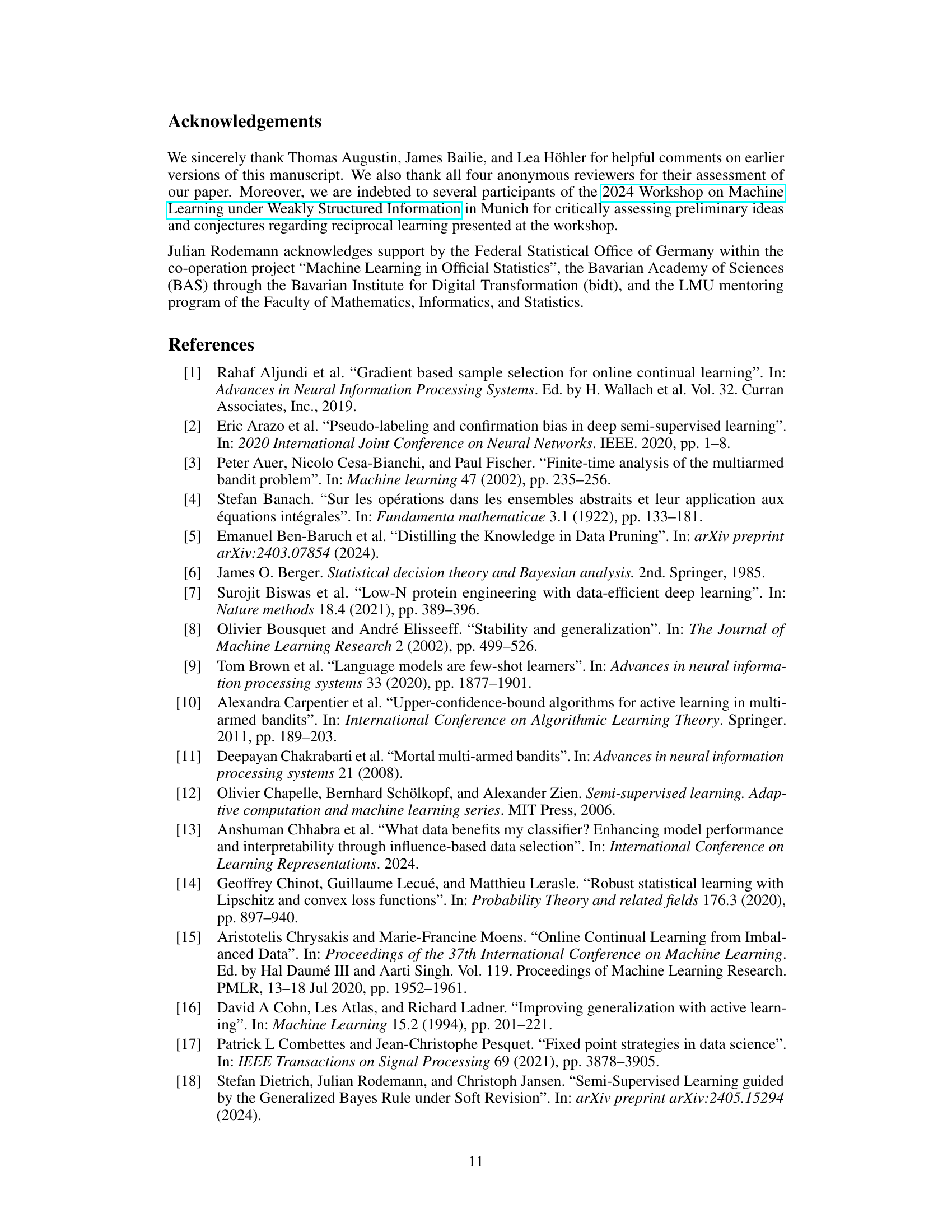
🔼 This figure illustrates a key concept in reciprocal learning: convergence. It shows an iterative process where a model is fitted to a sample (blue-grey circles), and then the sample is modified based on the model fit. The purple arrows represent changes in the sample space across iterations, while yellow arrows represent changes in the model space. The red curve represents the boundary of the model space, and the light grey area represents the sample space. The black dot represents the ’truth’. The figure demonstrates that for the algorithm to converge, the change in the sample (purple arrows) must be bounded by a constant multiple (L) of the combined change in the model and the previous sample (yellow arrows). This is expressed mathematically as d(P’’, P’’’) ≤ L.d((θ, P), (θ’, P’)). This inequality highlights that the algorithm’s stability relies on controlling data adaptation (the purple arrows) to prevent instability from disproportionate changes in the model and the data.
read the caption
Figure 3: Reciprocal learning converges if the change in sample (purple) is bounded by the change in model (yellow) and previous sample.
🔼 This figure compares classical machine learning to reciprocal learning. Panel A shows how classical machine learning fits a model to a fixed sample of data. Panel B shows how reciprocal learning iteratively updates the data based on the current model fit. This illustrates the key difference between the two approaches and highlights the feedback loop that defines reciprocal learning.
read the caption
Figure 1: (A) Classical machine learning fits a model from the model space (restricted by red curve) to a realized sample from the sample space (blue-grey); figure replicated from 'The Elements of Statistical Learning' [31, Figure 7.2]. (B) In reciprocal learning, the realized sample is no longer static, but changes in response to the model fit. Grey ellipse indicates restriction of sample space in t = 2 through realization in t = 1. Sample in t thus depends on model in t – 1 and sample in t−1.

🔼 This figure illustrates the difference between classical machine learning and reciprocal learning. In classical machine learning (A), a model is fitted to a static dataset, while in reciprocal learning (B), the dataset is iteratively updated based on the model fit in each iteration, creating a feedback loop between model and data.
read the caption
Figure 1: (A) Classical machine learning fits a model from the model space (restricted by red curve) to a realized sample from the sample space (blue-grey); figure replicated from 'The Elements of Statistical Learning' [31, Figure 7.2]. (B) In reciprocal learning, the realized sample is no longer static, but changes in response to the model fit. Grey ellipse indicates restriction of sample space in t = 2 through realization in t = 1. Sample in t thus depends on model in t – 1 and sample in t−1.

🔼 This figure compares classical machine learning to reciprocal learning. Panel (a) shows classical machine learning where a model is fitted to a static dataset. Panel (b) shows reciprocal learning, where the model iteratively refines itself by modifying the training data based on its current fit. The grey ellipse in (b) highlights how the sample space is restricted by the model fit, demonstrating the feedback loop between model and data.
read the caption
Figure 1: (A) Classical machine learning fits a model from the model space (restricted by red curve) to a realized sample from the sample space (blue-grey); figure replicated from 'The Elements of Statistical Learning' [31, Figure 7.2]. (B) In reciprocal learning, the realized sample is no longer static, but changes in response to the model fit. Grey ellipse indicates restriction of sample space in t = 2 through realization in t = 1. Sample in t thus depends on model in t – 1 and sample in t−1.
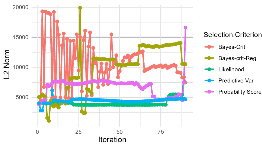
🔼 This figure compares the stability of the parameter vector (θt) in self-training with and without data regularization across different selection criteria. It shows the L2-norm of θt over iterations for three scenarios with varying proportions of unlabeled data (90%, 80%, and 70%). The results illustrate the stabilizing effect of data regularization, demonstrating that the regularized method is more stable than the unregularized method.
read the caption
Figure 6: Self-training with soft labels and varying selection criteria c(x, θ), one of which (Bayes-crit-reg) is regularized, on banknote data [21] with 70% (a) and 80% (b) unlabeled data; y-axis shows L2-Norm of θt at iteration t. Iterations vary between (a), (b), and (c) due to varying size of unlabeled data. Model: Generalized additive regression. Data source: Public UCI Machine Learning Repository [21]. References for other selection criteria: Bayes-crit: Rodemann, J., et al. 'Approximately Bayes-optimal pseudo-label selection.' [83]. Likelihood: Hüllermeier, E., Cheng, W. 'Superset learning based on generalized loss minimization.' [35] Predictive Var: Rizve, M, N., et al. 'In Defense of Pseudo-Labeling: An Uncertainty-Aware Pseudo-label Selection Framework for Semi-Supervised Learning.' [80]. Probability Score: Triguero, I., García, S., Herrera, F. (2015). 'Self-labeled techniques for semi-supervised learning: taxonomy, software and empirical study.' [103]. For details, see https://github.com/rodemann/simulations-self-training-reciprocal-learning.

🔼 This figure shows the L2 norm of the parameter vector in each iteration of self-training with different data selection criteria, both with and without regularization. The results are presented for datasets with varying proportions of unlabeled data (70%, 80%, and 90%). The figure illustrates the stabilizing effect of data regularization on the parameter vector.
read the caption
Figure 6: Self-training with soft labels and varying selection criteria c(x, θ), one of which (Bayes-crit-reg) is regularized, on banknote data [21] with 70% (a) and 80% (b) unlabeled data; y-axis shows L2-Norm of θt at iteration t. Iterations vary between (a), (b), and (c) due to varying size of unlabeled data. Model: Generalized additive regression. Data source: Public UCI Machine Learning Repository [21]. References for other selection criteria: Bayes-crit: Rodemann, J., et al. 'Approximately Bayes-optimal pseudo-label selection.' [83]. Likelihood: Hüllermeier, E., Cheng, W. 'Superset learning based on generalized loss minimization.' [35] Predictive Var: Rizve, M, N., et al. 'In Defense of Pseudo-Labeling: An Uncertainty-Aware Pseudo-label Selection Framework for Semi-Supervised Learning.' [80]. Probability Score: Triguero, I., García, S., Herrera, F. (2015). 'Self-labeled techniques for semi-supervised learning: taxonomy, software and empirical study.' [103]. For details, see https://github.com/rodemann/simulations-self-training-reciprocal-learning.

🔼 This figure compares the stability of the parameter vector in self-training with and without data regularization across various selection criteria. The L2-norm of the parameter vector is plotted against the iteration number for three different datasets (90%, 80%, and 70% unlabeled data).
read the caption
Figure 6: Self-training with soft labels and varying selection criteria c(x, θ), one of which (Bayes-crit-reg) is regularized, on banknote data [21] with 70% (a) and 80% (b) unlabeled data; y-axis shows L2-Norm of θt at iteration t. Iterations vary between (a), (b), and (c) due to varying size of unlabeled data. Model: Generalized additive regression. Data source: Public UCI Machine Learning Repository [21]. References for other selection criteria: Bayes-crit: Rodemann, J., et al. 'Approximately Bayes-optimal pseudo-label selection.' [83]. Likelihood: Hüllermeier, E., Cheng, W. 'Superset learning based on generalized loss minimization.' [35] Predictive Var: Rizve, M, N., et al. 'In Defense of Pseudo-Labeling: An Uncertainty-Aware Pseudo-label Selection Framework for Semi-Supervised Learning.' [80]. Probability Score: Triguero, I., García, S., Herrera, F. (2015). 'Self-labeled techniques for semi-supervised learning: taxonomy, software and empirical study.' [103]. For details, see https://github.com/rodemann/simulations-self-training-reciprocal-learning.
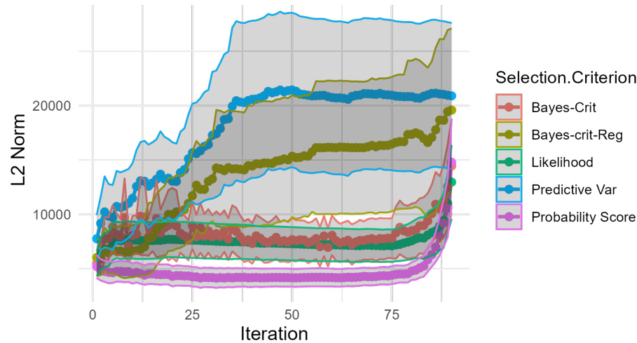
🔼 This figure displays the results of self-training experiments using various selection criteria, with one criterion being regularized. The y-axis shows the L2 norm of the parameter vector at each iteration, illustrating the stability of the model under different conditions. Three subfigures present results for datasets with varying amounts (70%, 80%, and 90%) of unlabeled data.
read the caption
Figure 6: Self-training with soft labels and varying selection criteria c(x, θ), one of which (Bayes-crit-reg) is regularized, on banknote data [21] with 70% (a) and 80% (b) unlabeled data; y-axis shows L2-Norm of θt at iteration t. Iterations vary between (a), (b), and (c) due to varying size of unlabeled data. Model: Generalized additive regression. Data source: Public UCI Machine Learning Repository [21]. References for other selection criteria: Bayes-crit: Rodemann, J., et al. 'Approximately Bayes-optimal pseudo-label selection.' [83]. Likelihood: Hüllermeier, E., Cheng, W. 'Superset learning based on generalized loss minimization.' [35] Predictive Var: Rizve, M, N., et al. 'In Defense of Pseudo-Labeling: An Uncertainty-Aware Pseudo-label Selection Framework for Semi-Supervised Learning.' [80]. Probability Score: Triguero, I., García, S., Herrera, F. (2015). 'Self-labeled techniques for semi-supervised learning: taxonomy, software and empirical study.' [103]. For details, see https://github.com/rodemann/simulations-self-training-reciprocal-learning.
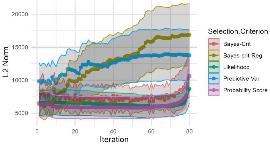
🔼 This figure compares the stability of the parameter vector (θₜ) in self-training with and without data regularization, using different selection criteria. It shows the L2 norm of θₜ over iterations for self-training on banknote data with varying amounts of unlabeled data (70%, 80%, and 90%). The results illustrate the stabilizing effect of data regularization on the parameter vector.
read the caption
Figure 6: Self-training with soft labels and varying selection criteria (c, cᵣ), one of which (Bayes-crit-reg) is regularized, on banknote data [21] with 70% (a) and 80% (b) unlabeled data; y-axis shows L2-Norm of θₜ at iteration t. Iterations vary between (a), (b), and (c) due to varying size of unlabeled data. Model: Generalized additive regression. Data source: Public UCI Machine Learning Repository [21]. References for other selection criteria: Bayes-crit: Rodemann, J., et al. 'Approximately Bayes-optimal pseudo-label selection.' [83]. Likelihood: Hüllermeier, E., Cheng, W. 'Superset learning based on generalized loss minimization.' [35] Predictive Var: Rizve, M, N., et al. 'In Defense of Pseudo-Labeling: An Uncertainty-Aware Pseudo-label Selection Framework for Semi-Supervised Learning.' [80]. Probability Score: Triguero, I., García, S., Herrera, F. (2015). 'Self-labeled techniques for semi-supervised learning: taxonomy, software and empirical study.' [103]. For details, see https://github.com/rodemann/simulations-self-training-reciprocal-learning.

🔼 The figure displays the L2 norm of the parameter vector (θt) over iterations for self-training with soft labels. It compares different data selection criteria, both regularized and unregularized, on banknote datasets with varying amounts of unlabeled data (70%, 80%, and 90%). The results illustrate the impact of data regularization on parameter stability.
read the caption
Figure 6: Self-training with soft labels and varying selection criteria c(x, θ), one of which (Bayes-crit-reg) is regularized, on banknote data [21] with 70% (a) and 80% (b) unlabeled data; y-axis shows L2-Norm of θt at iteration t. Iterations vary between (a), (b), and (c) due to varying size of unlabeled data. Model: Generalized additive regression. Data source: Public UCI Machine Learning Repository [21]. References for other selection criteria: Bayes-crit: Rodemann, J., et al. 'Approximately Bayes-optimal pseudo-label selection.' [83]. Likelihood: Hüllermeier, E., Cheng, W. 'Superset learning based on generalized loss minimization.' [35] Predictive Var: Rizve, M, N., et al. 'In Defense of Pseudo-Labeling: An Uncertainty-Aware Pseudo-label Selection Framework for Semi-Supervised Learning.' [80]. Probability Score: Triguero, I., García, S., Herrera, F. (2015). 'Self-labeled techniques for semi-supervised learning: taxonomy, software and empirical study.' [103]. For details, see https://github.com/rodemann/simulations-self-training-reciprocal-learning.
Full paper#
