TL;DR#
Zeroth-order optimization in machine learning (ML) aims to minimize loss functions without using gradient information, which is computationally expensive or unavailable in certain scenarios. Traditional boosting methods, while successful, often rely on first-order information (gradients), restricting their use to specific types of loss functions. A major limitation is that many existing zeroth-order methods require assumptions such as loss function convexity or differentiability for their convergence proofs to hold, which restricts their applicability to a subset of loss functions.
This research introduces a novel boosting algorithm, SECBOOST, which directly tackles these limitations. SECBOOST uses v-derivatives (a generalization of derivatives from quantum calculus) and Bregman secant distortions to optimize loss functions without any assumptions regarding differentiability or convexity. This is a major advancement as it significantly extends the applicability of boosting to a broader range of loss functions commonly encountered in ML problems. The algorithm introduces a new “offset oracle” component to further enhance its convergence properties. The theoretical analysis proves that SECBOOST converges to an optimal solution and provides a formal framework for understanding boosting without the reliance on traditional assumptions.
Key Takeaways#
Why does it matter?#
This paper is crucial because it addresses a long-standing challenge in machine learning (ML): efficiently optimizing any loss function using boosting, a technique traditionally limited by assumptions about loss function properties. Its findings broaden the applicability of boosting and provide new insights into zeroth-order optimization, paving the way for more efficient algorithms across various ML tasks.
Visual Insights#

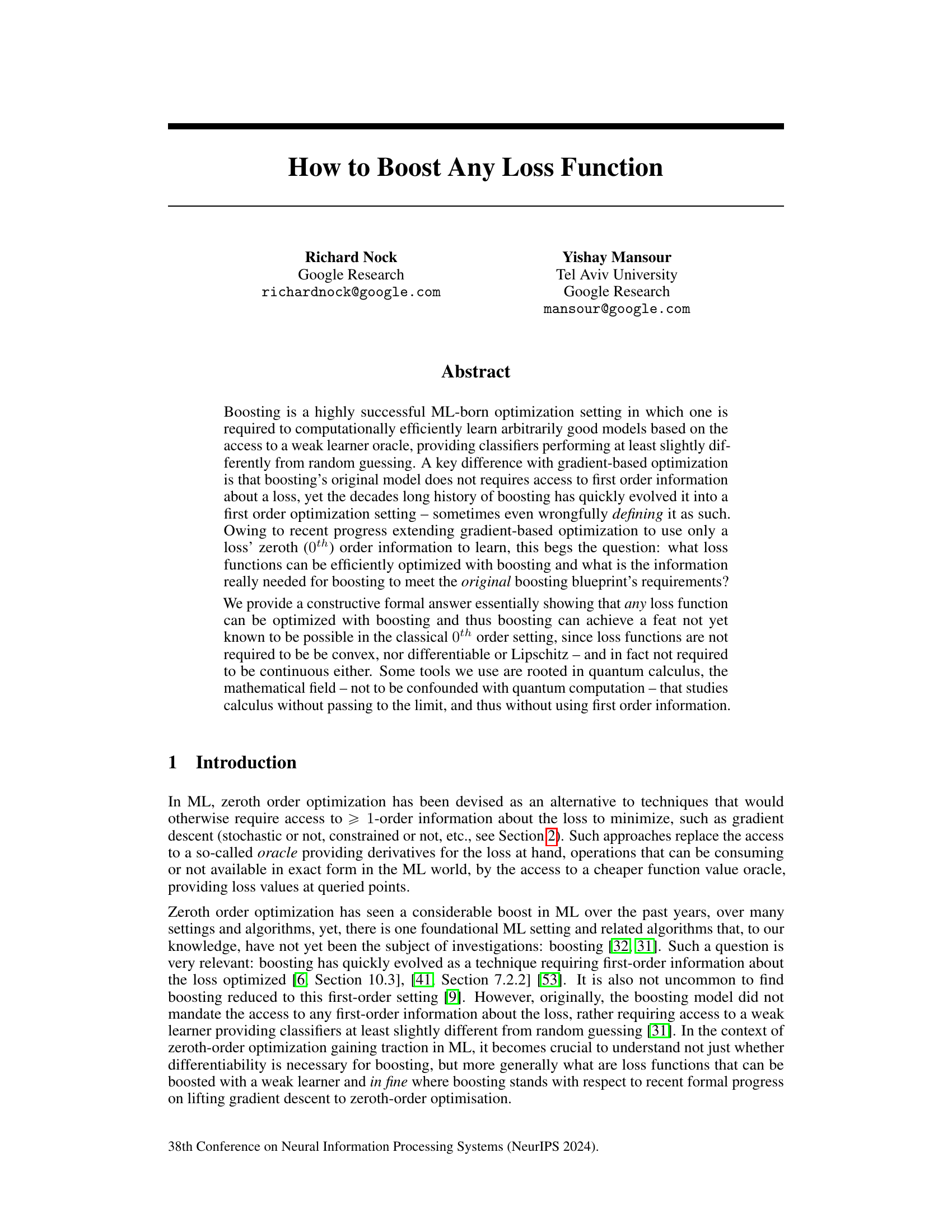
🔼 The left panel shows the Bregman Secant distortion for a convex function F. The distortion is positive, negative, minimal or null depending on the choice of z’. The right panel shows the Optimal Bregman Information (OBI) for a non-convex function F, illustrating the concept of the maximal difference between the line passing through (a,F(a)) and (b, F(b)) and the function F in the interval [a,c].
read the caption
Figure 1: Left: value of SF|v(z'||z) for convex F, v = z4 − z and various z' (colors), for which the Bregman Secant distortion is positive (z' = z1, green), negative (z' = z2, red), minimal (z' = z3) or null (z' = z4, z). Right: depiction of QF(z, z + v, z') for non-convex F (Definition 4.6).
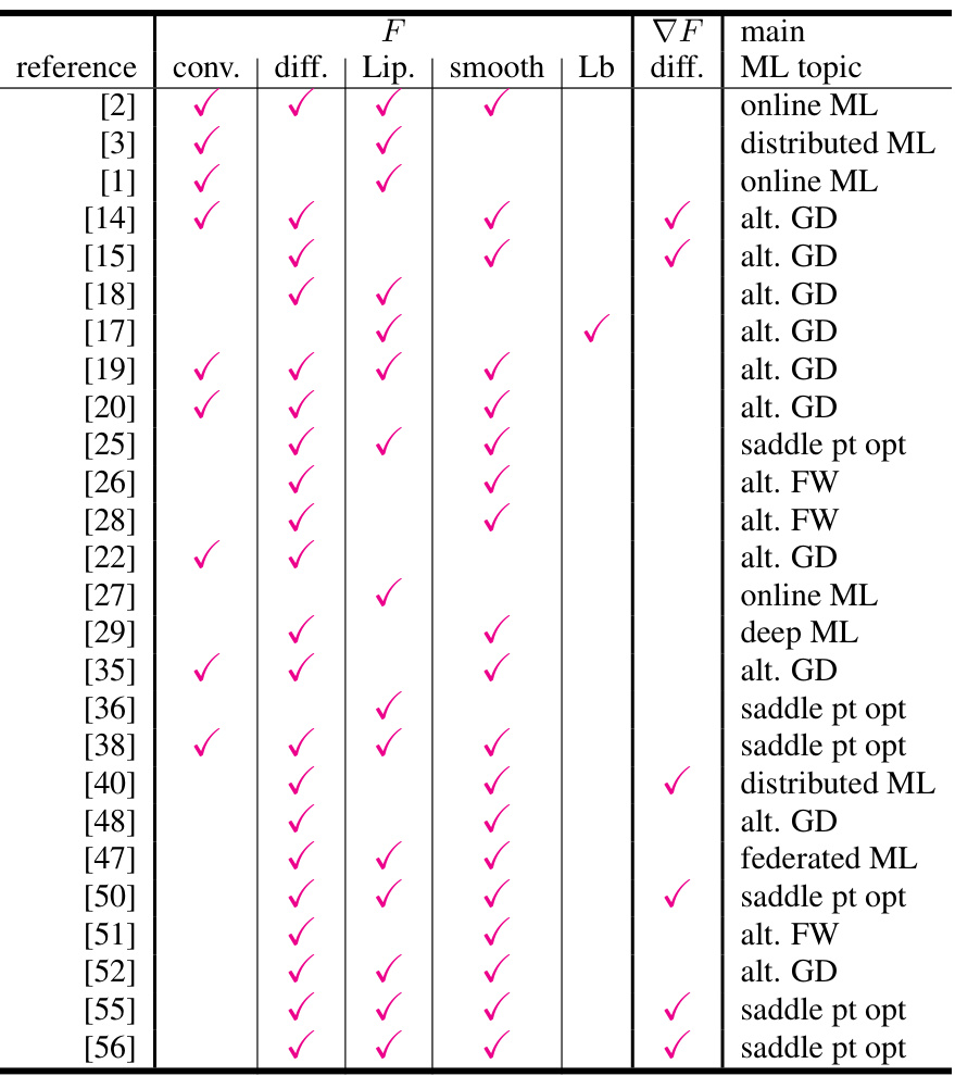
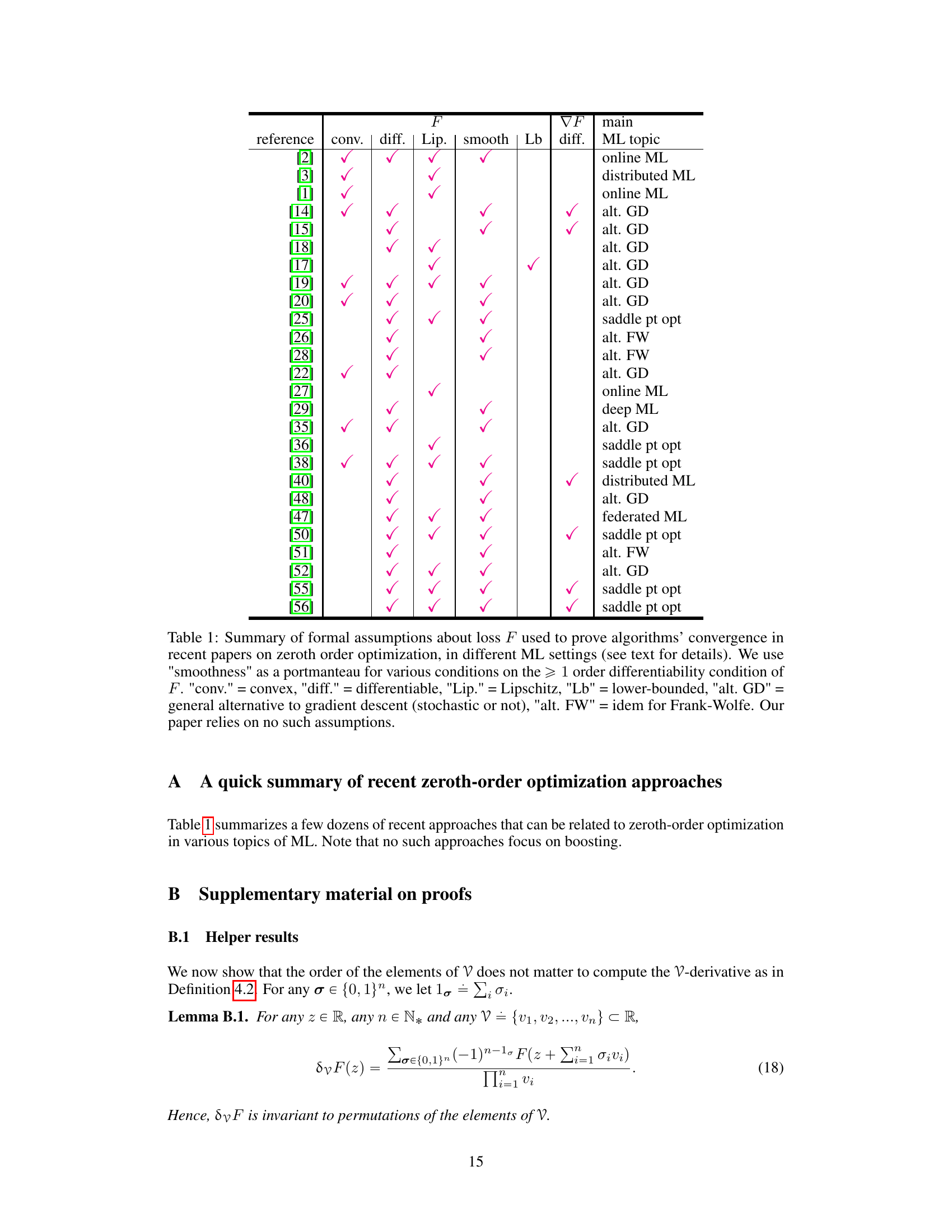
🔼 This table summarizes the assumptions made on the loss function (F) in various recent zeroth-order optimization algorithms. It compares different properties of the loss functions, such as convexity, differentiability, Lipschitz continuity, and smoothness. The table also indicates whether the algorithms are focused on online ML, distributed ML, saddle point optimization, or use alternative methods such as Frank-Wolfe. The key takeaway is that the current paper’s algorithm makes no assumptions about the loss function.
read the caption
Table 1: Summary of formal assumptions about loss F used to prove algorithms' convergence in recent papers on zeroth order optimization, in different ML settings (see text for details). We use 'smoothness' as a portmanteau for various conditions on the ≥ 1 order differentiability condition of F. 'conv.' = convex, 'diff.' = differentiable, 'Lip.' = Lipschitz, 'Lb' = lower-bounded, 'alt. GD' = general alternative to gradient descent (stochastic or not), 'alt. FW' = idem for Frank-Wolfe. Our paper relies on no such assumptions.
In-depth insights#
Boosting’s evolution#
Boosting, initially conceived as an optimization technique relying solely on a weak learner oracle, has significantly evolved over time. Early boosting algorithms didn’t require first-order information (gradients) about the loss function; their progress relied on comparing classifiers’ performance to random guessing. However, modern boosting methods heavily leverage gradient-based optimization, sometimes incorrectly categorized as first-order methods. This shift raises crucial questions about the fundamental information required for boosting’s success and which loss functions are amenable to this approach. Recent advancements in zeroth-order optimization, using only function values, have sparked renewed interest in boosting’s original, gradient-free formulation. The exploration of this intersection offers exciting possibilities for extending boosting beyond its traditional gradient-dependent frameworks, potentially unlocking efficient optimization strategies for a broader range of loss functions.
Zeroth-order methods#
Zeroth-order optimization methods are gradient-free techniques that estimate gradients using only function values, unlike traditional methods which require explicit gradient calculations. This is particularly useful in scenarios where gradients are unavailable, computationally expensive, or noisy. These methods leverage finite difference approximations or random search strategies to approximate the gradient, enabling optimization of non-differentiable or even discontinuous functions. A key advantage is their applicability to black-box optimization problems, where the underlying function’s structure is unknown. However, zeroth-order methods typically exhibit slower convergence rates compared to first-order methods due to the inherent noise in gradient estimation. Recent advancements have improved efficiency through sophisticated sampling strategies and advanced techniques like stochastic gradient estimations and momentum-based approaches. Despite the convergence challenges, zeroth-order methods remain a powerful tool for tackling optimization tasks in various domains, including machine learning, robotics, and control systems. The choice between zeroth-order and higher-order methods depends on a trade-off between computational cost and convergence speed, with the former favored in high-dimensional settings or when gradient information is unreliable.
SECBOOST algorithm#
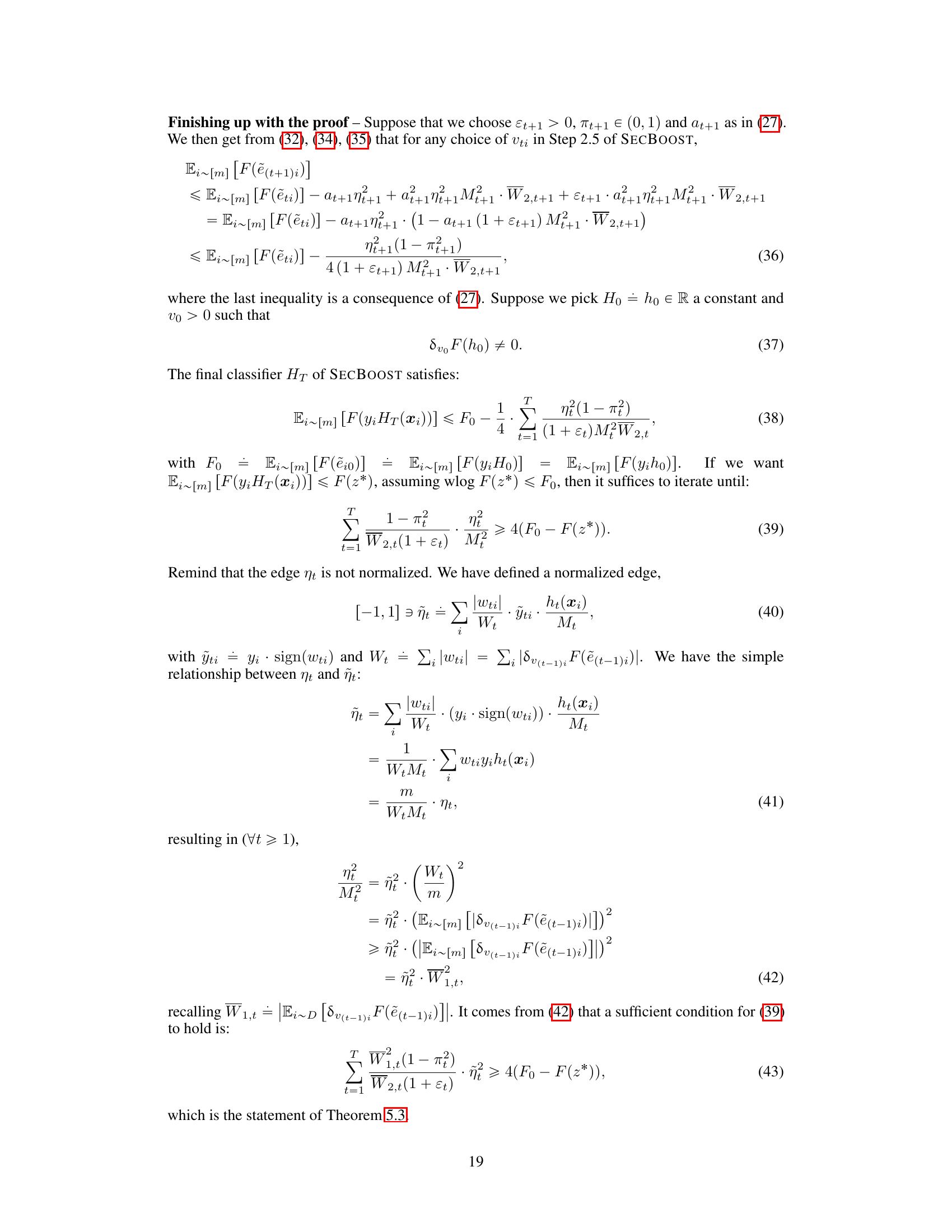
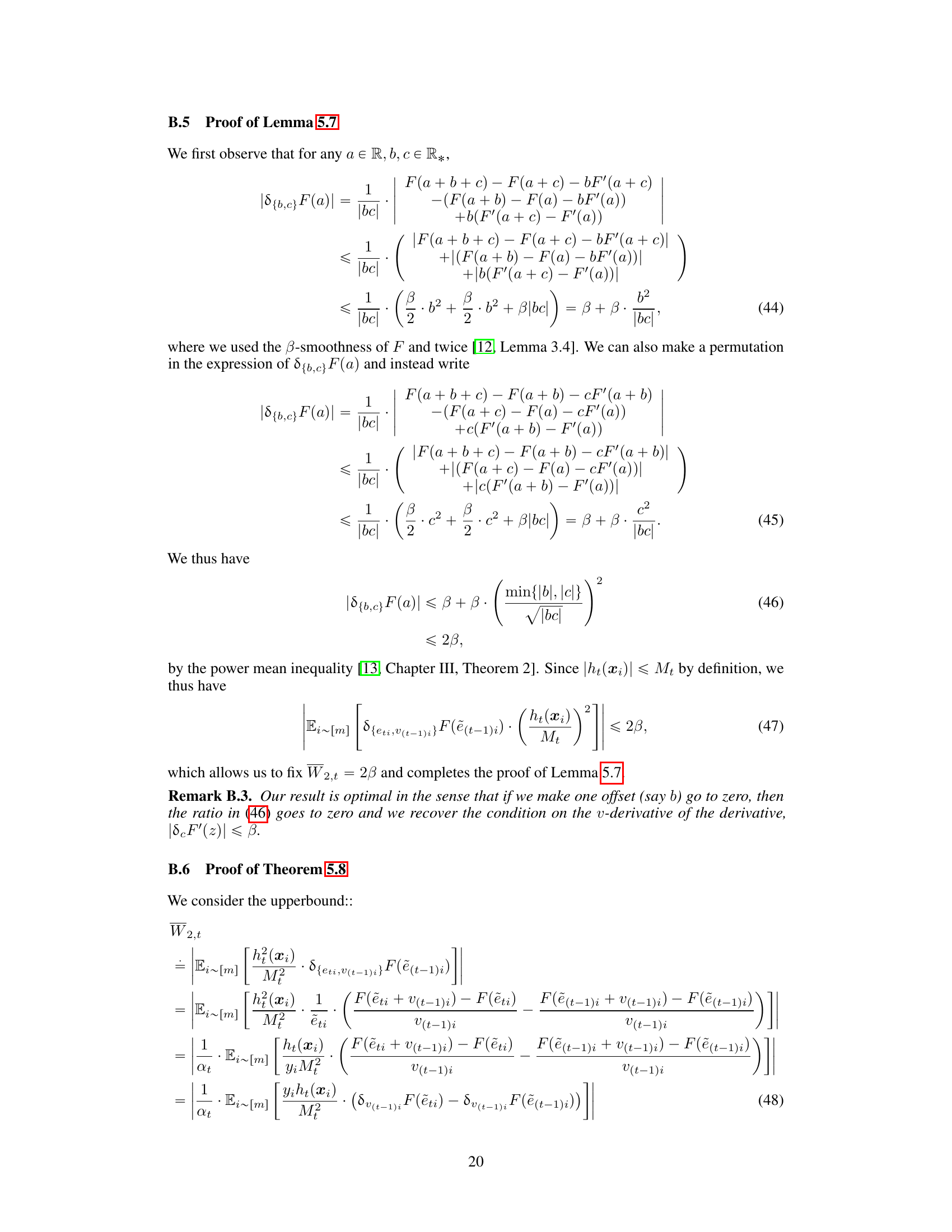
The SECBOOST algorithm is a novel approach to boosting that significantly departs from traditional methods by eliminating the need for first-order information (derivatives) about the loss function. It leverages zeroth-order information, specifically loss function values, and a weak learner oracle to iteratively construct a strong classifier. The algorithm introduces the concept of offset oracles which compute suitable offsets for the loss function approximations, enabling it to operate even on discontinuous, non-convex, and non-Lipschitz loss functions. A key strength is its theoretical guarantee of convergence, even under relaxed weak learning assumptions, without imposing stringent conditions on the loss function’s properties, as commonly seen in traditional zeroth-order optimization algorithms. This expands the scope of boosting’s applicability to a much wider range of ML problems. The algorithm uses v-derivatives and a generalized Bregman information to quantify progress in each boosting iteration, providing a novel theoretical foundation. Its flexibility in choosing leveraging coefficients and offsets allows adaptability to the loss function’s characteristics and leads to a trade-off between computational efficiency and convergence speed.
Convergence analysis#
A rigorous convergence analysis is crucial for any machine learning algorithm, and this paper is no exception. The authors delve into the convergence properties of their novel boosting algorithm, demonstrating that it can efficiently optimize a wide range of loss functions. Key aspects of their analysis involve the use of v-derivatives and Bregman secant distortions. This approach moves beyond traditional zeroth-order optimization methods that often rely on stringent assumptions like convexity or differentiability. The analysis elegantly links the algorithm’s convergence rate to the weak learning assumption’s advantage over random guessing, a cornerstone of boosting theory. The introduction of the offset oracle adds a layer of complexity to the analysis, but it also plays a critical role in ensuring the algorithm’s convergence guarantees. The analysis highlights a balance between the flexibility in choosing parameters and the strength of the convergence guarantees, suggesting that careful parameter tuning is necessary for optimal performance. Overall, the convergence analysis provides strong theoretical underpinnings for the practical effectiveness of the boosting algorithm, showcasing its ability to handle a broader class of loss functions than previously explored.
Future work#
The paper’s “Future Work” section could explore several promising avenues. Extending the algorithm’s applicability to a broader range of loss functions is crucial, potentially investigating non-convex, non-differentiable, or even discontinuous functions beyond those already addressed. A deeper investigation into the offset oracle’s impact on convergence is also warranted, possibly exploring adaptive or learned offset selection strategies. Analyzing the algorithm’s generalization performance on larger, more complex datasets would provide valuable insights into its real-world applicability. Moreover, exploring connections with other zeroth-order optimization techniques would help position the proposed method within the broader optimization landscape. Finally, developing practical implementation strategies that balance theoretical optimality with computational efficiency would be beneficial for wider adoption.
More visual insights#
More on figures

🔼 This figure illustrates different scenarios for the quantity W2,t in Assumption 5.5, which is related to the variation of weights in the boosting algorithm. Panel (a) shows a ’nice’ loss function where W2,t remains small. Panels (b) through (d) depict scenarios where a ‘bump’ in the loss function can cause W2,t to become large. Panels (c) and (d) propose strategies to mitigate this issue either by selecting smaller offsets or using larger offsets to bypass the problematic area.
read the caption
Figure 2: Simplified depiction of W2,t 'regimes' (Assumption 5.5). We only plot the components of the v-derivative part in (8): removing index i for readability, we get d{et,vt−1}F(ēt−1) = (Bt − At)/(yHt(x) − yHt−1(x)) with At = δvt−1F(yHt−1(x)) = −wt and Bt = δvt−1F(yHt(x)) (= −wt+1 iff vt−1 = vt). If the loss is 'nice' like the exponential or logistic losses, we always have a small W2,t (a). Place a bump in the loss (b-d) and the risk happens that W2,t is too large for the WRA to hold. Workarounds include two strategies: picking small enough offsets (b) or fit offsets large enough to pass the bump (c). The blue arrow in (d) is discussed in Section 6.

🔼 This figure illustrates a simple method to construct the set Iti(z) for a discontinuous loss function F. The method involves rotating two half-lines and identifying points where one line intersects the function F while the other remains below F. The process generates candidate offsets (v) that are collected to form the final set Iti(z).
read the caption
Figure 3: A simple way to build Iti(z) for a discontinuous loss F (ēti < ē(t−1)i and z are represented), O being the set of solutions as it is built. We rotate two half-lines, one passing through (ēti, F(ēti)) (thick line, (△)) and a parallel one translated by -z (dashed line) (a). As soon as (∆) crosses F on any point (z', F(z')) with z ≠ ěti while the dashed line stays below F, we obtain a candidate offset v for OO, namely v = z' – ěti. In (b), we obtain an interval of values. We keep on rotating (Δ), eventually making appear several intervals for the choice of v if F is not convex (c). Finally, when we reach an angle such that the maximal difference between (△) and F in [ēti, ē(t−1)i] is z (z can be located at an intersection between F and the dashed line), we stop and obtain the full Iti(z) (d).

🔼 This figure illustrates a simple method for constructing the set Iti(z) for a discontinuous loss function F. The method involves rotating two half-lines and identifying points where one half-line intersects the function F while the other remains below F. The process iteratively builds the set Iti(z) by identifying candidate offsets, and the complete set is obtained when the maximum difference between one half-line and F reaches the target value z. The figure showcases the construction process for both convex and non-convex functions, highlighting how the structure of Iti(z) can vary.
read the caption
Figure 3: A simple way to build Iti(z) for a discontinuous loss F (ēti < ē(t−1)i and z are represented), O being the set of solutions as it is built. We rotate two half-lines, one passing through (ēti, F(ēti)) (thick line, (△)) and a parallel one translated by -z (dashed line) (a). As soon as (∆) crosses F on any point (z', F(z')) with z ≠ ěti while the dashed line stays below F, we obtain a candidate offset v for OO, namely v = z' – ěti. In (b), we obtain an interval of values. We keep on rotating (Δ), eventually making appear several intervals for the choice of v if F is not convex (c). Finally, when we reach an angle such that the maximal difference between (△) and F in [ēti, ē(t−1)i] is z (z can be located at an intersection between F and the dashed line), we stop and obtain the full Iti(z) (d).

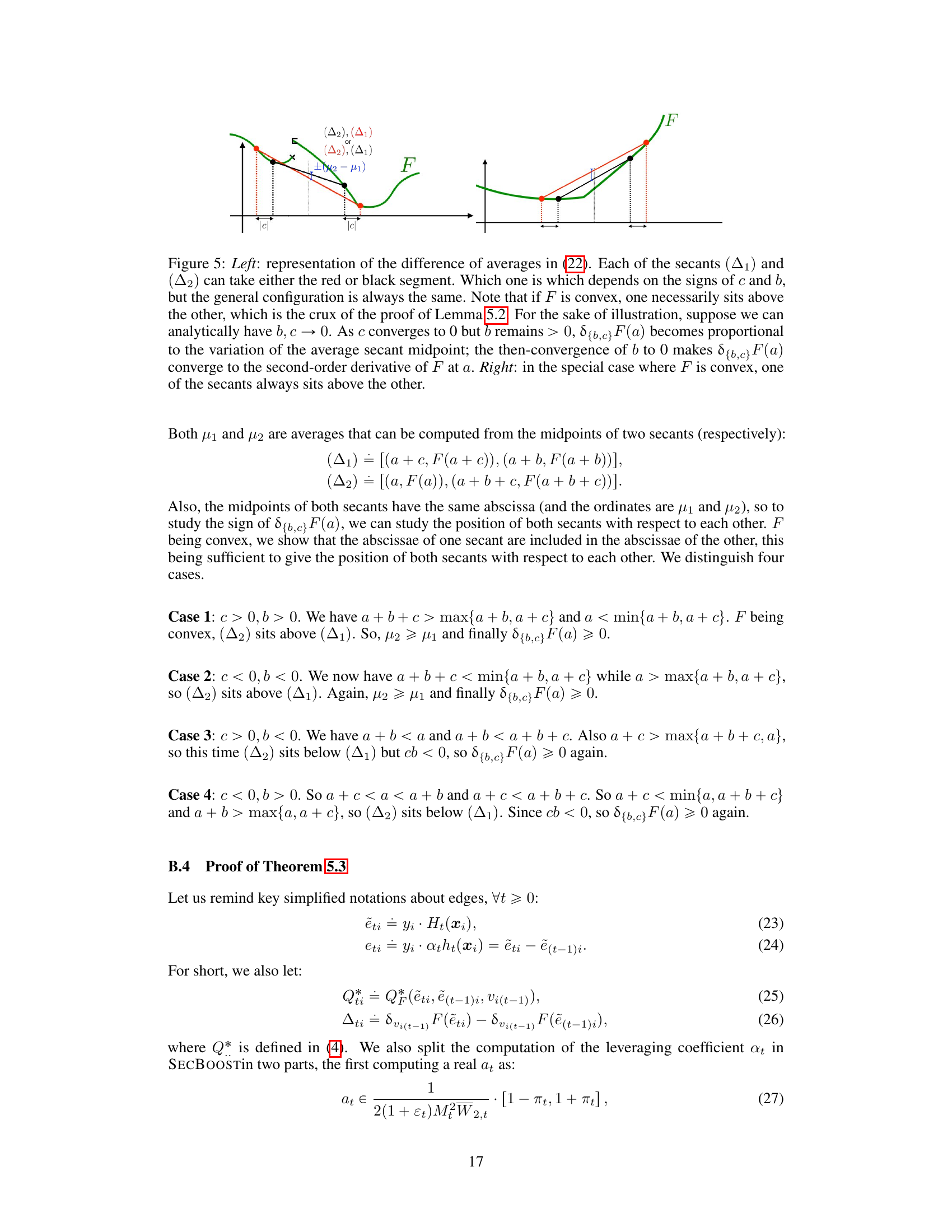
🔼 The figure demonstrates the relationship between the Bregman Secant distortions and Bregman divergences. The left panel shows how the difference of averages in equation (22) is related to the secants (△₁) and (△2). It illustrates that if the function F is convex, one secant will always sit above the other. The right panel focuses on the specific case where F is convex, emphasizing that one secant will always sit above the other. This geometric illustration helps to explain why the Bregman Secant distortion is a useful generalization of the Bregman divergence.
read the caption
Figure 5: Left: representation of the difference of averages in (22). Each of the secants (△₁) and (A2) can take either the red or black segment. Which one is which depends on the signs of c and b, but the general configuration is always the same. Note that if F is convex, one necessarily sits above the other, which is the crux of the proof of Lemma 5.2. For the sake of illustration, suppose we can analytically have b, c → 0. As c converges to 0 but b remains > 0, 8{b,c}F(a) becomes proportional to the variation of the average secant midpoint; the then-convergence of b to 0 makes d{b,c}F(a) converge to the second-order derivative of F at a. Right: in the special case where F is convex, one of the secants always sits above the other.
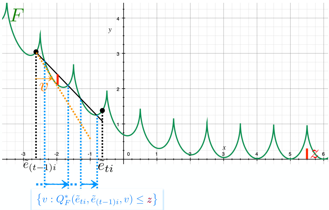
🔼 Figure 6 shows a spring loss function, which is neither convex, nor Lipschitz, nor differentiable and has infinitely many local minima. Despite this, a trivial implementation of the offset oracle is possible. The orange line segment illustrates how a single tangent point can be computed to obtain the offset, simplifying the offset oracle computation.
read the caption
Figure 6: The spring loss in (53) is neither convex, nor Lipschitz or differentiable and has an infinite number of local minima. Yet, an implementation of the offset oracle is trivial as an output for OO can be obtained from the computation of a single tangent point (here, the orange v, see text; best viewed in color).
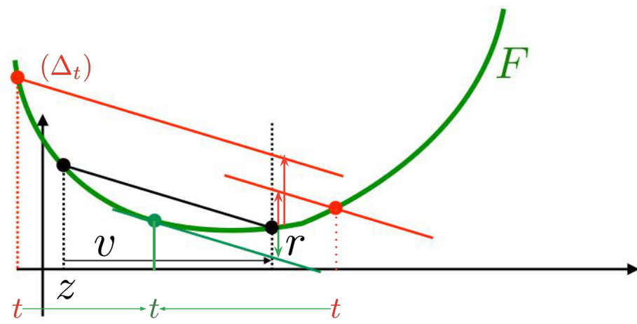
🔼 This figure illustrates how to compute the Optimal Bregman Information (OBI) for a convex function F. It shows how to find the value of v that maximizes the difference between the secant connecting points (z, F(z)) and (z+v, F(z+v)) and the function F itself within the interval [z, z+v]. The optimal value of v is found when the maximal difference between the secant and the function is equal to r.
read the caption
Figure 7: Computing the OBI QF(z, z + v, z + v) for F convex, (z, v) being given and v > 0. We compute the line (△t) crossing F at any point t, with slope equal to the secant [(z, F(z)), (z + v, F(z + v))] and then the difference between F at z + v and this line at z + v. We move t so as to maximize this difference. The optimal t (in green) gives the corresponding OBI. In (56) and (58), we are interested in finding v given this difference, r. We also need to replicate this computation for v < 0.
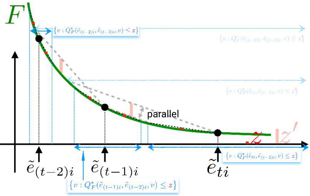
🔼 This figure shows two scenarios for a strictly convex function F. The first scenario (smaller z) demonstrates that if the intervals generated by the algorithm (Iti(z)) are disjoint, then the weights will decrease monotonically with each iteration, following standard boosting behavior. The second scenario (larger z’) illustrates that if the intervals are not disjoint, then this weight decrease is not guaranteed and the weights may increase in subsequent iterations.
read the caption
Figure 8: Case F strictly convex, with two cases of limit OBI z and z' in Iti(.). Example i has eti > 0 and ẽ(t−1)i > 0 (??) large enough (hence, edges with respect to weak classifiers ht and ht−1 large enough) so that Iti(z) ∩ I(t−1)i(z) = I(t−1)i(z) ∩ I(t−2)i(z) = Iti(z) ∩ Ⅱ(t−2)i(z) = Ø. In this case, regardless of the offsets chosen by 00, we are guaranteed that its weights satisfy W(t+1)i < Wti < W(t−1)i, which follows the boosting pattern that examples receiving the right classification by weak classifiers have their weights decreasing. If however the limit OBI changes from z to a larger z', this is not guaranteed anymore: in this case, it may be the case that w(t+1)i > Wti.
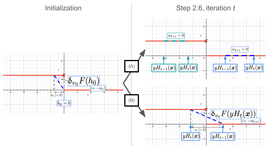
🔼 Figure 9 shows how the algorithm handles the 0/1 loss. Initialization gives all examples positive weights. During weight updates, if the strong model’s edge remains the same sign (positive or negative), the next weight will be 0. If the signs are different, the next weight will be non-zero.
read the caption
Figure 9: How our algorithm works with the 0/1 loss (in red): at the initialization stage, assuming we pick ho = 0 for simplicity and some vo < 0, all training examples get the same weight, given by negative the slope of the thick blue dashed line. All weights are thus > 0. At iteration t when we update the weights (Step 2.6), one of two cases can happen on some training example (x, y). In (A), the edge of the strong model remains the same: either both are positive (blue) or both negative (olive green) (the ordering of edges is not important). In this case, regardless of the offset, the new weight will be 0. In (B), both edges have different sign (again, the ordering of edges is not important). In this case, the examples will keep non-zero weight over the next iteration. See text below for details.

🔼 This figure illustrates a method for building the set Iti(z) for a discontinuous loss function F. The method involves rotating two half-lines, one passing through (ēti, F(ēti)) and the other translated by -z, and identifying points where the first half-line intersects F while the second remains below F. Each intersection point provides a candidate offset v. The process continues until the maximal difference between the rotated half-line and F within the interval [ēti, ē(t−1)i] equals z. The resulting set of offsets v forms Iti(z). Different panels show the process for various stages and conditions.
read the caption
Figure 3: A simple way to build Iti(z) for a discontinuous loss F (ēti < ē(t−1)i and z are represented), O being the set of solutions as it is built. We rotate two half-lines, one passing through (ēti, F(ēti)) (thick line, (△)) and a parallel one translated by -z (dashed line) (a). As soon as (△) crosses F on any point (z', F(z')) with z' ≠ ěti while the dashed line stays below F, we obtain a candidate offset v for OO, namely v = z' – ěti. In (b), we obtain an interval of values. We keep on rotating (Δ), eventually making appear several intervals for the choice of v if F is not convex (c). Finally, when we reach an angle such that the maximal difference between (△) and F in [ēti, ē(t−1)i] is z (z can be located at an intersection between F and the dashed line), we stop and obtain the full Iti(z) (d).
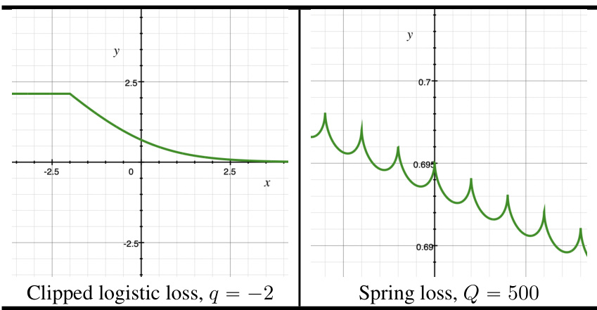
🔼 The figure shows plots of two loss functions used in the experiments: the clipped logistic loss and the spring loss. These loss functions are compared to the standard logistic loss to highlight their non-standard properties (non-convexity, non-differentiability, etc.). The figure provides visual context for the challenges presented by these loss functions in the optimization experiments described in the paper.
read the caption
Figure 11: Crops of the two losses whose optimization has been experimentally tested with SEC-BOOST, in addition to the logistic loss. See text for details.
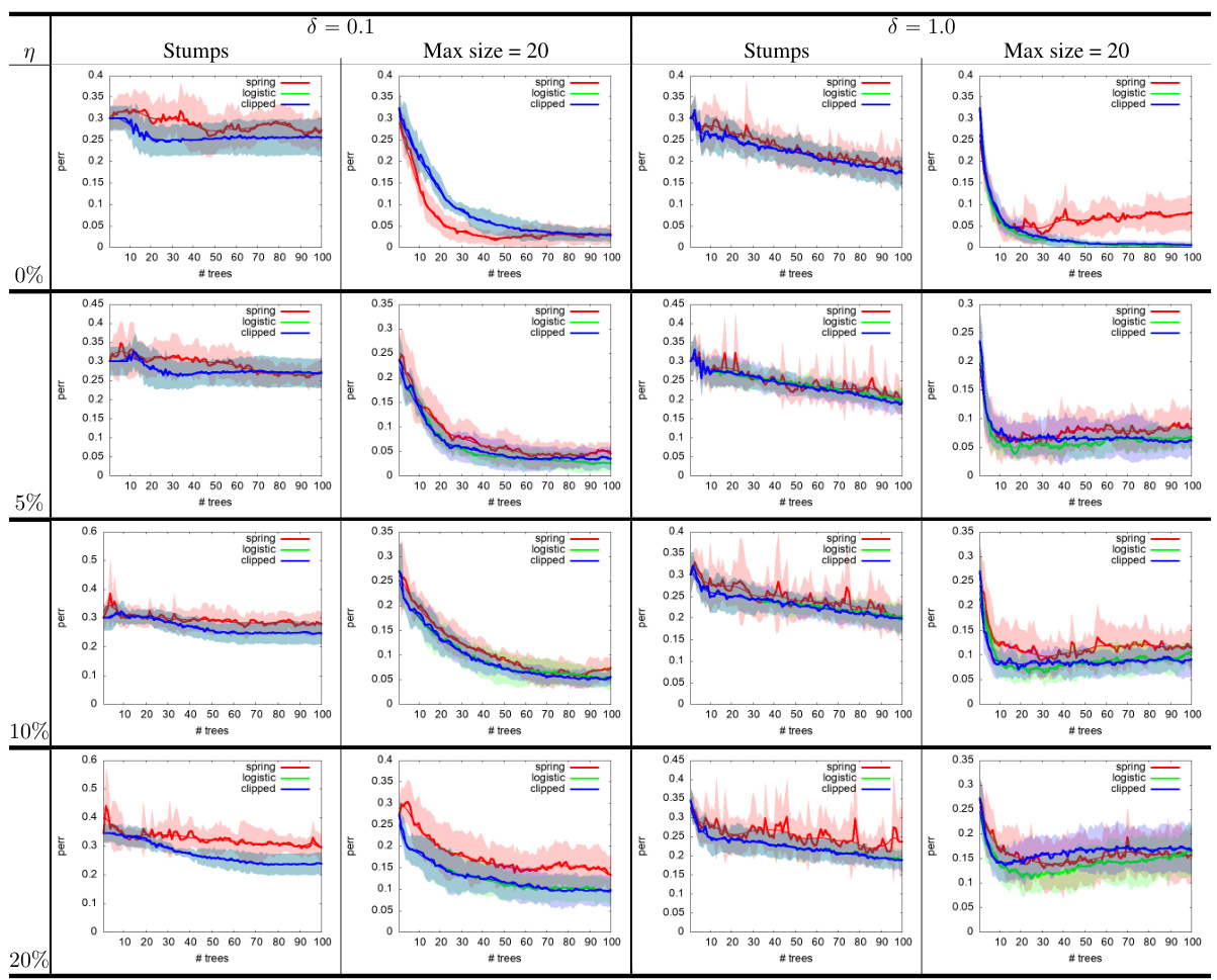
🔼 This figure displays the results of experiments conducted on the UCI tic-tac-toe dataset using the SECBOOST algorithm. The experiments compare the performance of SECBOOST when minimizing three different loss functions: the logistic loss, the clipped logistic loss, and the spring loss. The results are shown for different levels of training noise (η), maximum tree size, and initial hyperparameter (δ). Each combination of parameters is represented by a different colored line and shaded region. The shaded regions represent the confidence intervals of the results. The x-axis represents the number of trees used in the boosting algorithm and y-axis represents the test error rate.
read the caption
Figure 12: Experiments on UCI tictactoe showing estimated test errors after minimizing each of the three losses we consider, with varying training noise level η, max tree size and initial hyperparameter δ value in (60). See text.
Full paper#
