TL;DR#
Traditional numerical methods for solving partial differential equations (PDEs) are computationally expensive, requiring fine meshes and small time steps. Machine learning offers an alternative, but existing methods often suffer from issues like poor interpretability, weak generalizability, and high dependence on large labeled datasets. This paper introduces a new approach to address these limitations.
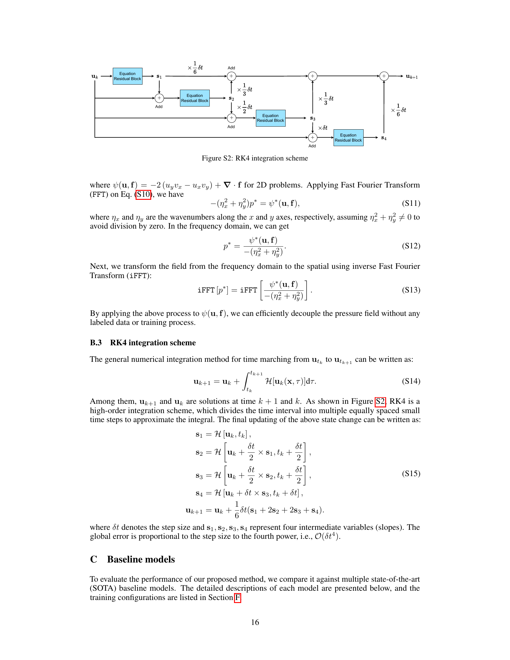
The proposed model, P2C2Net, uses a physics-encoded approach, combining a trainable PDE block with a neural network correction module. The PDE block updates the solution based on a high-order scheme, while the neural network block corrects for errors introduced by the coarse grid. The model employs a learnable symmetric convolutional filter for accurate derivative estimation. Experiments show that P2C2Net achieves state-of-the-art performance and generalizability across various datasets, even with limited training data, significantly outperforming existing methods.
Key Takeaways#
Why does it matter?#
This paper is important because it presents P2C2Net, a novel and efficient method for predicting spatiotemporal dynamics using limited data. This addresses a critical challenge in solving partial differential equations (PDEs), where high-resolution methods are computationally expensive and data-hungry methods lack generalizability. P2C2Net’s ability to handle coarse grids and small datasets opens new avenues for research in various fields involving complex dynamical systems. Its superior performance and efficiency demonstrated across multiple datasets make it a significant contribution to the field.
Visual Insights#
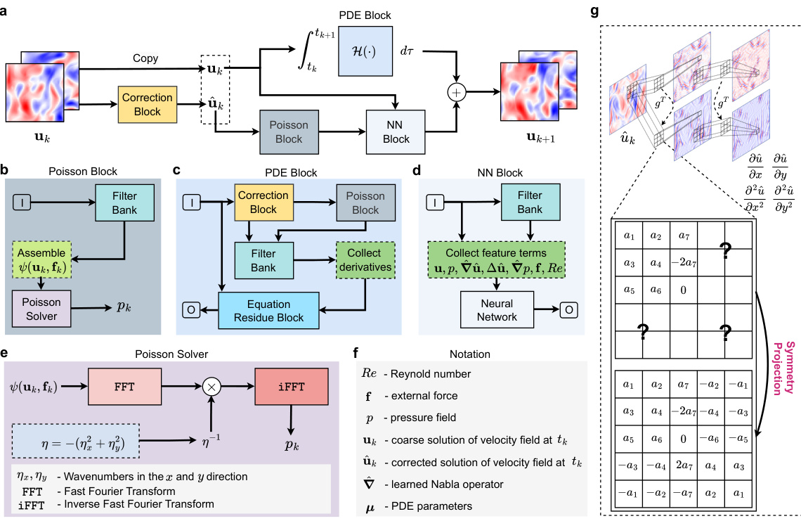
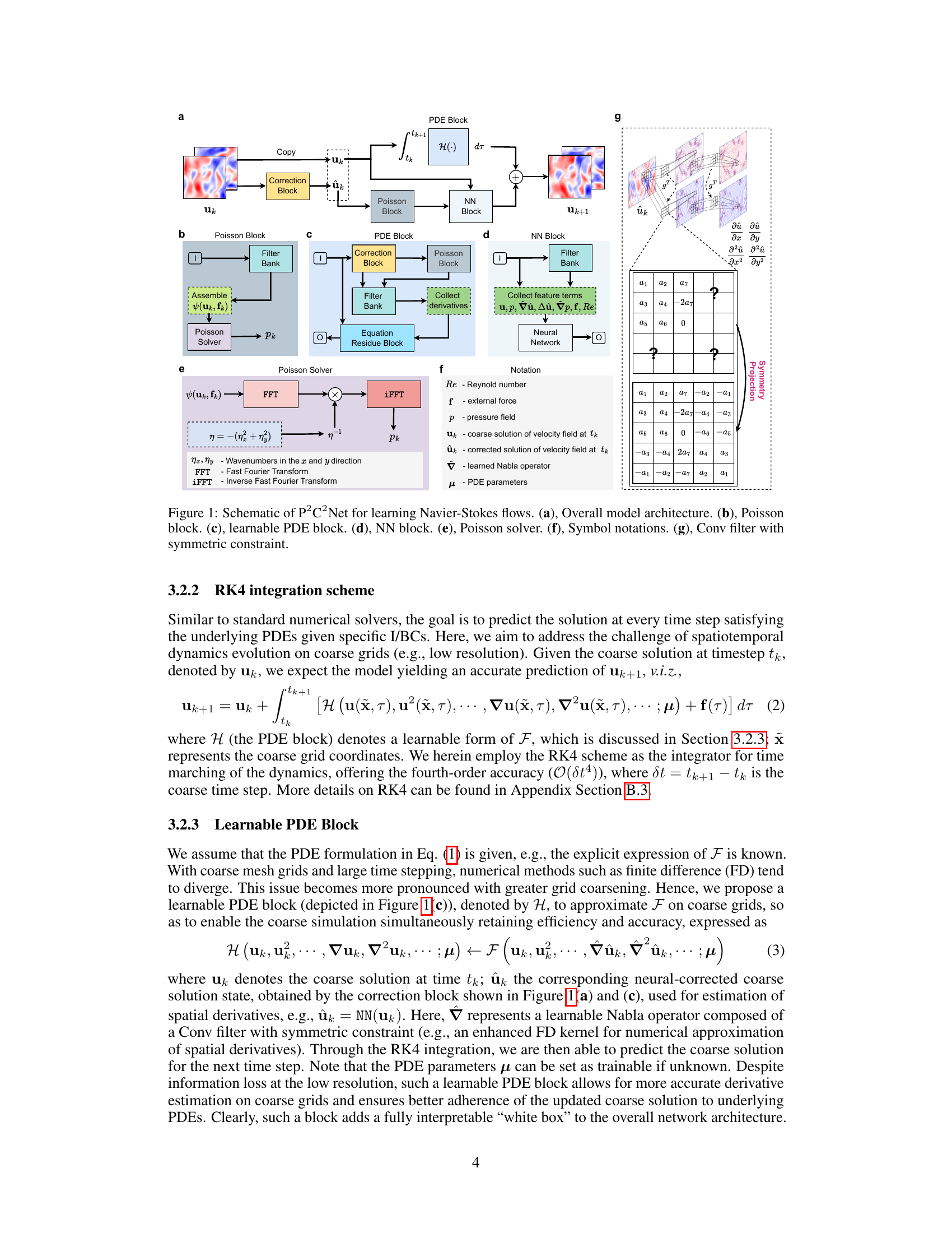
🔼 This figure shows the architecture of the P2C2Net model for learning Navier-Stokes flows. It’s broken down into several blocks: the overall architecture (a), the Poisson block (b), the learnable PDE block (c), the NN block (d), the Poisson solver (e), symbol notations (f), and a convolution filter with symmetric constraints (g). Each block plays a crucial role in the process of efficiently predicting complex spatiotemporal dynamics, especially on coarse grids. The model uses a combination of classical numerical methods and learnable neural network components to achieve accuracy and efficiency in solving partial differential equations.
read the caption
Figure 1: Schematic of P2C2Net for learning Navier-Stokes flows. (a), Overall model architecture. (b), Poisson block. (c), learnable PDE block. (d), NN block. (e), Poisson solver. (f), Symbol notations. (g), Conv filter with symmetric constraint.
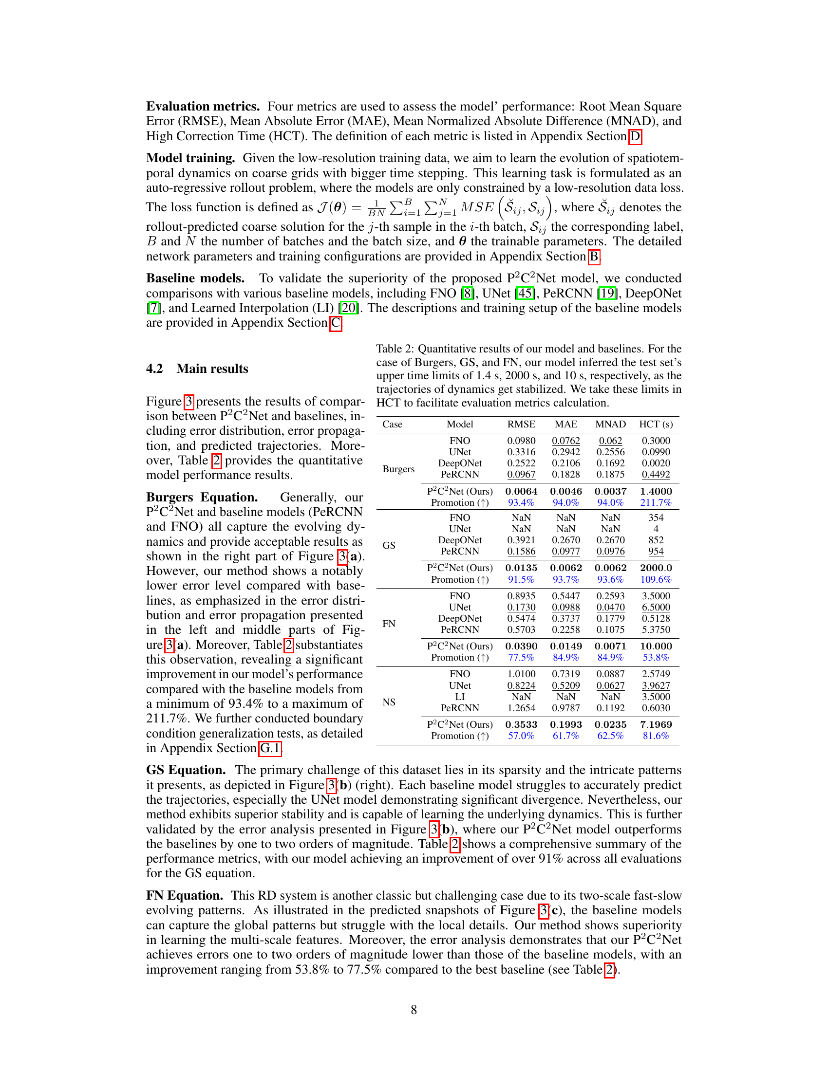
🔼 This table summarizes the datasets used in the paper for training and testing the proposed model. It shows the numerical method used to generate the data (FD for finite difference, FV for finite volume), the spatial and temporal grid resolutions (both original and downsampled for training), the number of training and testing trajectories, and the number of rollout steps for testing. The datasets cover various complex PDE problems.
read the caption
Table 1: Summary of datasets and training implementations. Note that '→' denotes the downsampling process from the original resolution (simulation) to the low resolution (training).
In-depth insights#
PDE-Aware Networks#
PDE-aware networks represent a significant advancement in the field of scientific machine learning, bridging the gap between traditional numerical methods for solving partial differential equations (PDEs) and the flexibility of deep learning. These networks integrate physical knowledge encoded in PDEs directly into their architectures, improving accuracy, generalization, and data efficiency. This integration can manifest in several ways, such as incorporating PDE residuals into the loss function, enforcing boundary conditions explicitly, or designing network layers that directly approximate PDE operators. A key advantage is the ability to handle complex, high-dimensional PDEs, often intractable with purely numerical methods. However, challenges remain in terms of interpretability and the need for careful design to ensure stability and convergence. Furthermore, the reliance on sufficient training data can still limit the applicability of some PDE-aware networks; therefore, research into techniques that leverage small datasets and incorporate prior knowledge more effectively remains an active area of exploration. Ultimately, these networks hold immense potential for accelerating scientific discovery and engineering design by offering computationally efficient and physically consistent solutions to complex PDE problems.
Coarse Grid Learning#
Coarse grid learning tackles the challenge of efficiently solving partial differential equations (PDEs) by leveraging coarser spatial and temporal resolutions than traditional methods. This approach reduces computational costs significantly, making it particularly appealing for high-dimensional or computationally intensive problems. The key trade-off lies in the potential loss of accuracy due to reduced resolution. Therefore, successful coarse grid learning methods often incorporate techniques to mitigate this loss, such as incorporating prior physical knowledge into the model (physics-informed learning), using advanced neural network architectures to learn complex mappings between coarse and fine scales, or employing a hybrid approach that combines learned components with classical numerical schemes. Effective coarse grid learning requires careful consideration of the balance between computational efficiency and solution accuracy. The effectiveness of this approach depends heavily on the nature of the PDE, the specific application, and the choice of learning techniques. Research in this area often focuses on developing novel neural network architectures, regularisation techniques, or data augmentation strategies. The overall goal is to create reliable and efficient algorithms that provide accurate approximations of PDE solutions while significantly reducing computational complexity.
Conv Filter Design#
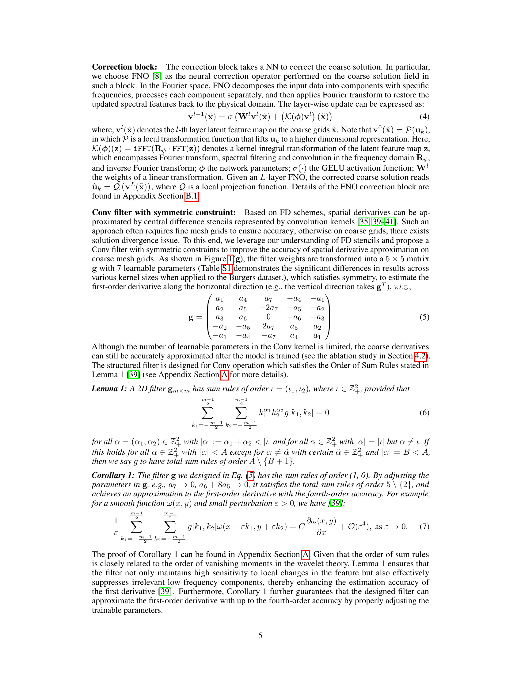
The design of convolutional filters is crucial for accurately estimating spatial derivatives in Partial Differential Equation (PDE) solvers, particularly when operating on coarse grids. A naive approach using standard finite difference stencils can lead to instability and inaccuracy due to the reduced resolution. Therefore, a learnable symmetric convolutional filter is proposed, using a small number of trainable parameters to approximate derivatives effectively. This approach is motivated by the observation that symmetric stencils naturally enhance estimation accuracy. The filter’s design incorporates a constraint which ensures it satisfies a desired order of sum rules, guaranteeing high accuracy even on coarse grids. This design choice is especially beneficial in data-scarce scenarios, enhancing the overall model’s performance and interpretability by leveraging the structured information inherent in the filter. The learnable nature of the filter further allows the model to adapt to specific PDE characteristics and datasets, thereby optimizing its performance on complex spatiotemporal dynamics. The use of a symmetric filter avoids numerical instability and ensures improved solution accuracy and generalization ability compared to using asymmetric filters or traditional numerical methods alone.
Generalization Tests#
Generalization tests in machine learning assess a model’s ability to perform well on unseen data that differs from the training data. Robust generalization is crucial for reliable model deployment because real-world data is rarely perfectly representative of the training set. In the context of Partial Differential Equation (PDE) solvers, generalization means the model accurately predicts the system’s behavior across various initial conditions (ICs), boundary conditions (BCs), parameters, and even different PDEs. Successfully generalizing to unseen PDEs demonstrates the model has learned fundamental physical principles rather than simply memorizing training examples. Testing generalization often involves evaluating performance across ranges of parameter values, different initial states, and varying types of PDEs. Strong generalization indicates the model is learning the underlying physics rather than overfitting to the specific training data. Therefore, these tests are vital in demonstrating a PDE solver’s practical applicability and reliability.
Future Directions#
Future research directions for PDE-solving neural networks like P2C2Net could focus on several key areas. Extending the model to handle more complex geometries and boundary conditions beyond simple periodic boundaries is crucial for real-world applicability. This might involve exploring mesh-based methods or graph neural networks to handle irregular domains. Improving the efficiency and scalability of the model for high-dimensional problems is another vital direction, requiring investigation of novel architectures and more efficient training techniques. Addressing the issue of limited training data remains a challenge; future work should explore techniques like data augmentation, transfer learning, or active learning to improve generalizability. Developing methods for uncertainty quantification to provide confidence intervals around predictions is also critical for trust and reliability, particularly in safety-critical applications. Finally, exploring the integration of physics-informed neural networks with other AI techniques like reinforcement learning could lead to innovative solutions for complex spatiotemporal dynamics prediction and control.
More visual insights#
More on figures

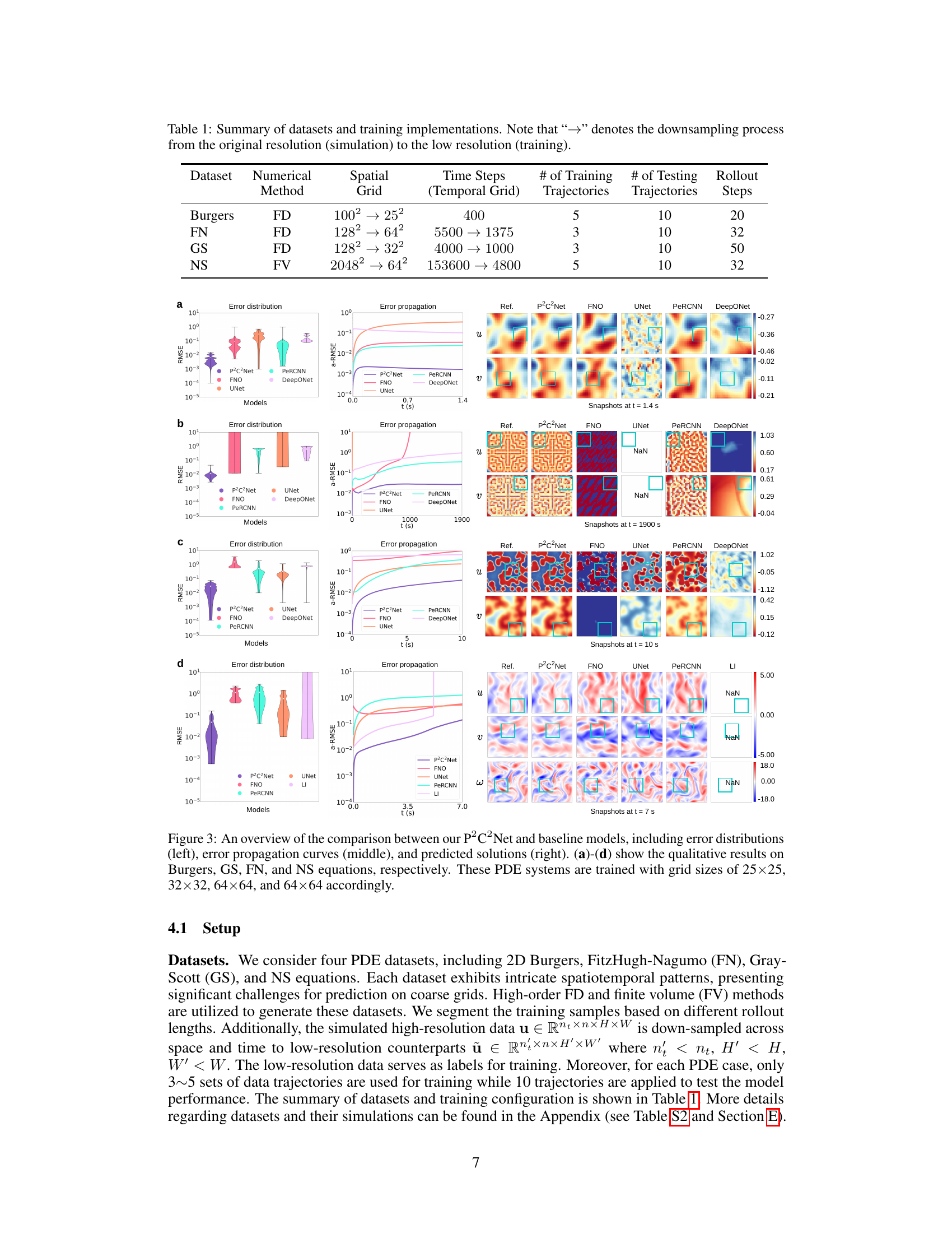
🔼 This figure presents a comparison of P2C2Net against several baseline models. The comparison includes four different partial differential equations (PDEs). For each PDE, the figure shows three plots: error distribution, error propagation curves, and snapshots of the predicted solutions. Error distribution shows the range of errors, error propagation shows how errors change over time, and snapshots show the visual representation of the predicted solutions. This figure aims to demonstrate the superiority of P2C2Net in terms of solution accuracy and generalization.
read the caption
Figure 3: An overview of the comparison between our P2C2Net and baseline models, including error distributions (left), error propagation curves (middle), and predicted solutions (right). (a)-(d) show the qualitative results on Burgers, GS, FN, and NS equations, respectively. These PDE systems are trained with grid sizes of 25×25, 32×32, 64×64, and 64×64 accordingly.

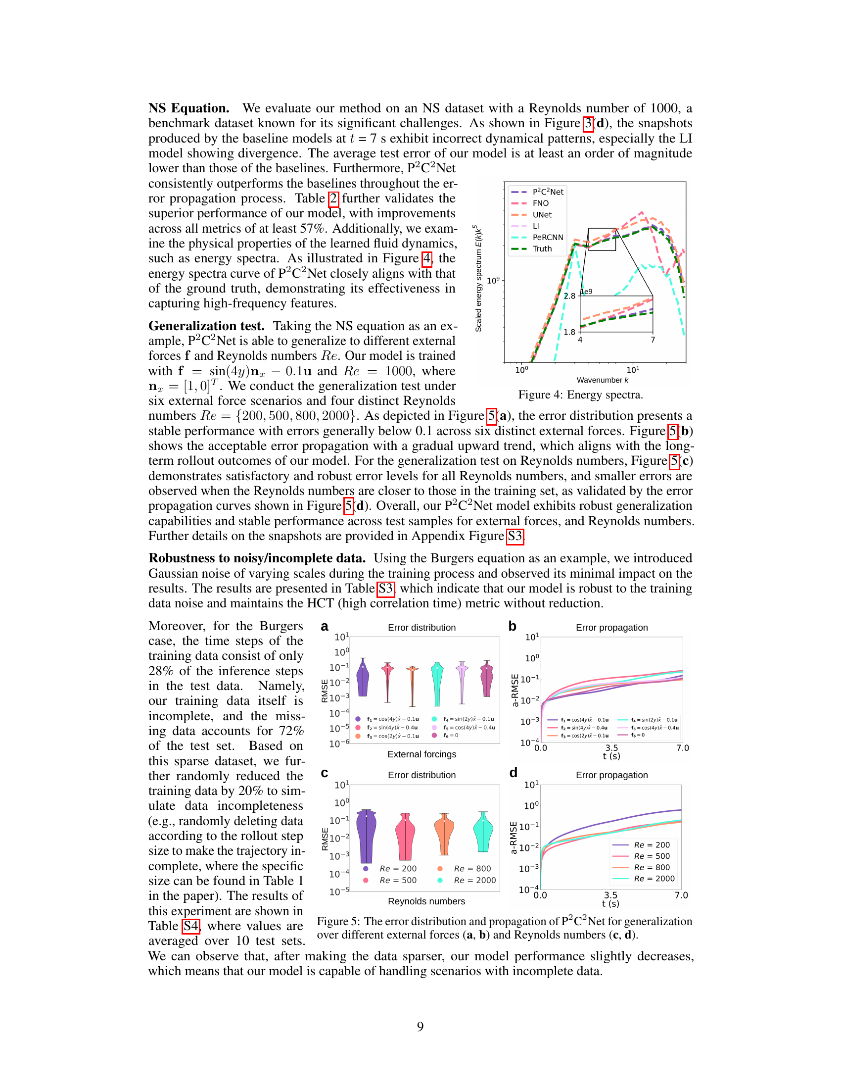
🔼 This figure compares the energy spectra of the proposed P2C2Net model against several baseline models, including FNO, UNet, LI, and PeRCNN, and the ground truth. The x-axis represents the wavenumber k, and the y-axis represents the scaled energy spectrum E(k)k⁵. The plot shows that the energy spectra of P2C2Net closely matches the ground truth across different wavenumbers. The inset is a zoomed-in view of the lower wavenumber region to better show the differences among the models.
read the caption
Figure 4: Energy spectra.
🔼 This figure presents a comparison of the proposed P2C2Net model against several baseline models across four different partial differential equation (PDE) systems. The comparison is shown through visualizations of error distributions, error propagation curves, and example solution snapshots. Four PDE systems are used, each with different levels of complexity, illustrating the performance of P2C2Net under varying conditions.
read the caption
Figure 3: An overview of the comparison between our P2C2Net and baseline models, including error distributions (left), error propagation curves (middle), and predicted solutions (right). (a)-(d) show the qualitative results on Burgers, GS, FN, and NS equations, respectively. These PDE systems are trained with grid sizes of 25×25, 32×32, 64×64, and 64×64 accordingly.
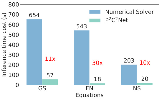
🔼 This bar chart compares the inference time cost (in seconds) between a numerical solver and the proposed P2C2Net model across three different partial differential equations (PDEs): Gray-Scott (GS), FitzHugh-Nagumo (FN), and Navier-Stokes (NS). For each PDE, the chart shows the time taken by the numerical solver and P2C2Net, highlighting the significant speedup achieved by P2C2Net. The speedup factors are explicitly indicated for each PDE. This figure illustrates the computational efficiency gains of the P2C2Net method.
read the caption
Figure 6: Computational time for comparison.
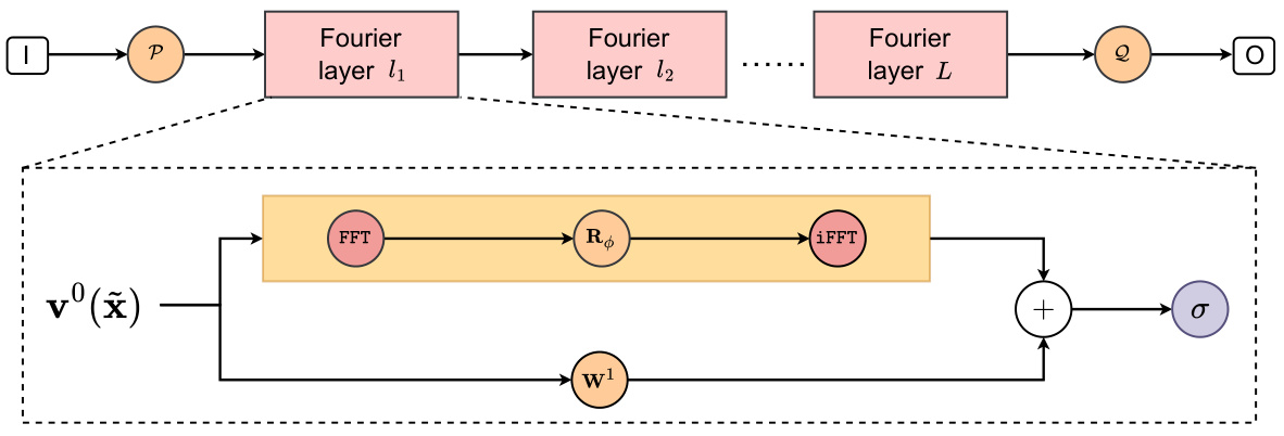
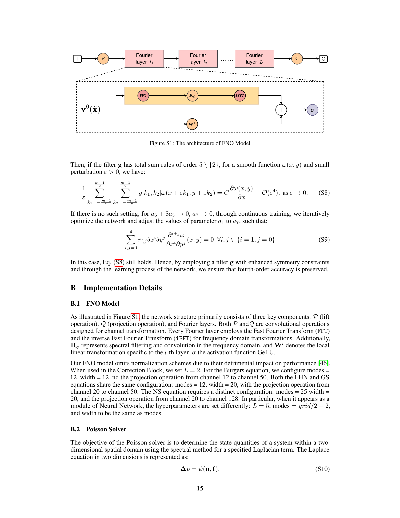
🔼 The figure illustrates the architecture of the Fourier Neural Operator (FNO) model. The FNO model consists of three main components: a lift operation (P), a projection operation (Q), and L Fourier layers. The lift operation transforms the input into a higher-dimensional representation. Each Fourier layer performs a Fast Fourier Transform (FFT), spectral filtering and convolution using Rθ, and an Inverse Fast Fourier Transform (iFFT), capturing both local and global features. The projection operation maps the output of the final Fourier layer back into the original data space. A linear transformation (Wl) and activation function (σ) are also included within each Fourier layer. The model is designed to handle inputs and outputs in the form of functions.
read the caption
Figure S1: The architecture of FNO Model

🔼 This figure shows the architecture of P2C2Net, a physics-encoded correction learning model for efficiently solving spatiotemporal PDE problems. It’s composed of four main blocks: a state variable correction block, a learnable PDE block, a Poisson block, and a neural network (NN) block. The figure details the data flow through these blocks, highlighting the learnable symmetric convolutional filter used for accurate spatial derivative estimation and the RK4 integration scheme for temporal evolution. Subfigures (a)-(g) break down the overall architecture and individual components.
read the caption
Figure 1: Schematic of P2C2Net for learning Navier-Stokes flows. (a), Overall model architecture. (b), Poisson block. (c), learnable PDE block. (d), NN block. (e), Poisson solver. (f), Symbol notations. (g), Conv filter with symmetric constraint.

🔼 This figure compares the performance of P2C2Net against other baseline models across four different PDE systems. It shows error distributions, error propagation curves, and example predictions for each model on the Burgers, Gray-Scott, FitzHugh-Nagumo, and Navier-Stokes equations. The training grid sizes varied depending on the equation. The results demonstrate P2C2Net’s superior performance in terms of accuracy and stability.
read the caption
Figure 3: An overview of the comparison between our P2C2Net and baseline models, including error distributions (left), error propagation curves (middle), and predicted solutions (right). (a)-(d) show the qualitative results on Burgers, GS, FN, and NS equations, respectively. These PDE systems are trained with grid sizes of 25×25, 32×32, 64×64, and 64×64 accordingly.
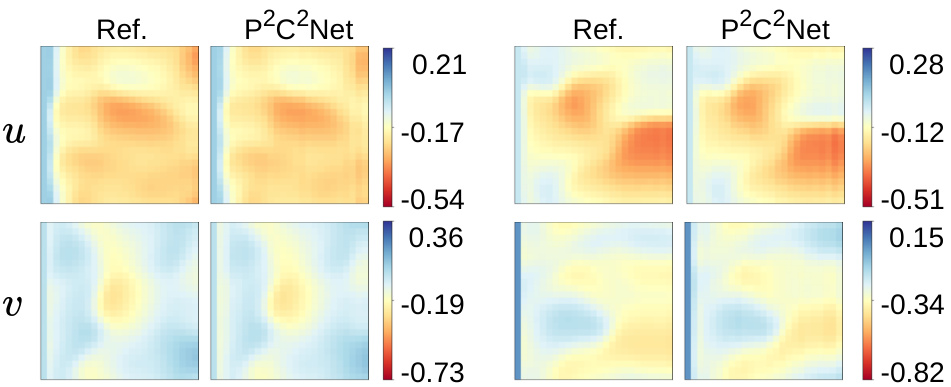
🔼 This figure presents a comparison of P2C2Net against several baseline models on four different PDE systems (Burgers, Gray-Scott, FitzHugh-Nagumo, and Navier-Stokes). For each PDE, it shows three subfigures: 1) Error Distribution: Illustrates the distribution of prediction errors, revealing the accuracy and robustness of each model. 2) Error Propagation: Plots the error propagation over time, providing insights into the stability and long-term prediction capability of the models. 3) Predicted Solutions: Visualizes the predicted solutions, comparing them qualitatively to the ground truth. The different subfigures (a-d) showcase the performance on varying PDE systems trained on different grid resolutions.
read the caption
Figure 3: An overview of the comparison between our P2C2Net and baseline models, including error distributions (left), error propagation curves (middle), and predicted solutions (right). (a)-(d) show the qualitative results on Burgers, GS, FN, and NS equations, respectively. These PDE systems are trained with grid sizes of 25×25, 32×32, 64×64, and 64×64 accordingly.
More on tables

🔼 This table summarizes the datasets used in the paper’s experiments. It shows the numerical methods used to generate the data (FD for finite difference, FV for finite volume), the spatial and temporal grid resolutions (before and after downsampling), the number of training and testing trajectories, and the number of rollout steps in each testing trajectory. The downsampling from higher resolution simulation data to lower resolution training data is indicated by the ‘→’ symbol.
read the caption
Table 1: Summary of datasets and training implementations. Note that '→' denotes the downsampling process from the original resolution (simulation) to the low resolution (training).

🔼 This table presents a quantitative comparison of the proposed P2C2Net model’s performance against several baseline models across different PDE datasets (Burgers, GS, FN, NS). The metrics used for comparison include RMSE, MAE, MNAD, and HCT (High Correction Time). The HCT values for Burgers, GS, and FN reflect the point where the dynamics stabilize. The ‘Promotion’ row indicates the percentage improvement achieved by P2C2Net over the best-performing baseline model for each metric.
read the caption
Table 2: Quantitative results of our model and baselines. For the case of Burgers, GS, and FN, our model inferred the test set's upper time limits of 1.4 s, 2000 s, and 10 s, respectively, as the trajectories of dynamics get stabilized. We take these limits in HCT to facilitate evaluation metrics calculation.
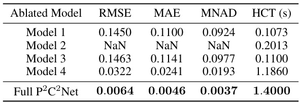
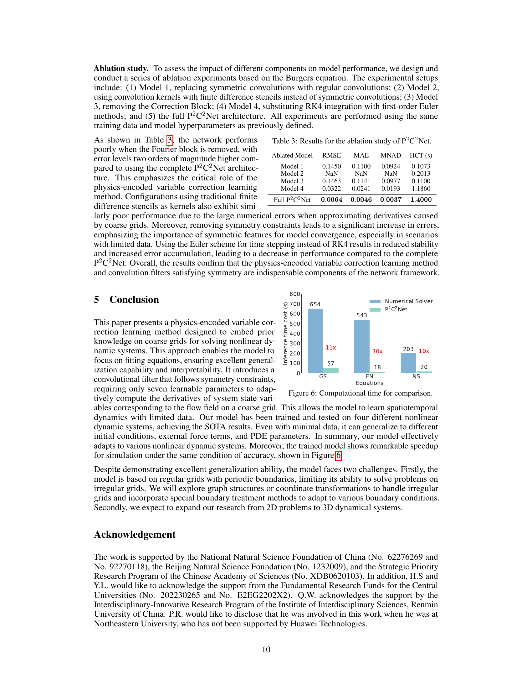
🔼 This table presents a quantitative analysis of the ablation study conducted on the P2C2Net model for the Burgers equation. Five different models were evaluated: Model 1 (replacing symmetric convolutions with regular convolutions), Model 2 (using convolution kernels with finite difference stencils), Model 3 (removing the Correction Block), Model 4 (substituting RK4 integration with first-order Euler methods), and the full P2C2Net architecture. The performance of each model is assessed using four metrics: RMSE, MAE, MNAD, and HCT. The results clearly demonstrate the importance of the symmetric convolutional filter, the correction block, and the high-order RK4 integration scheme for achieving high accuracy in solving the Burgers equation.
read the caption
Table 3: Results for the ablation study of P2C2Net.
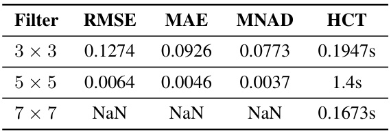
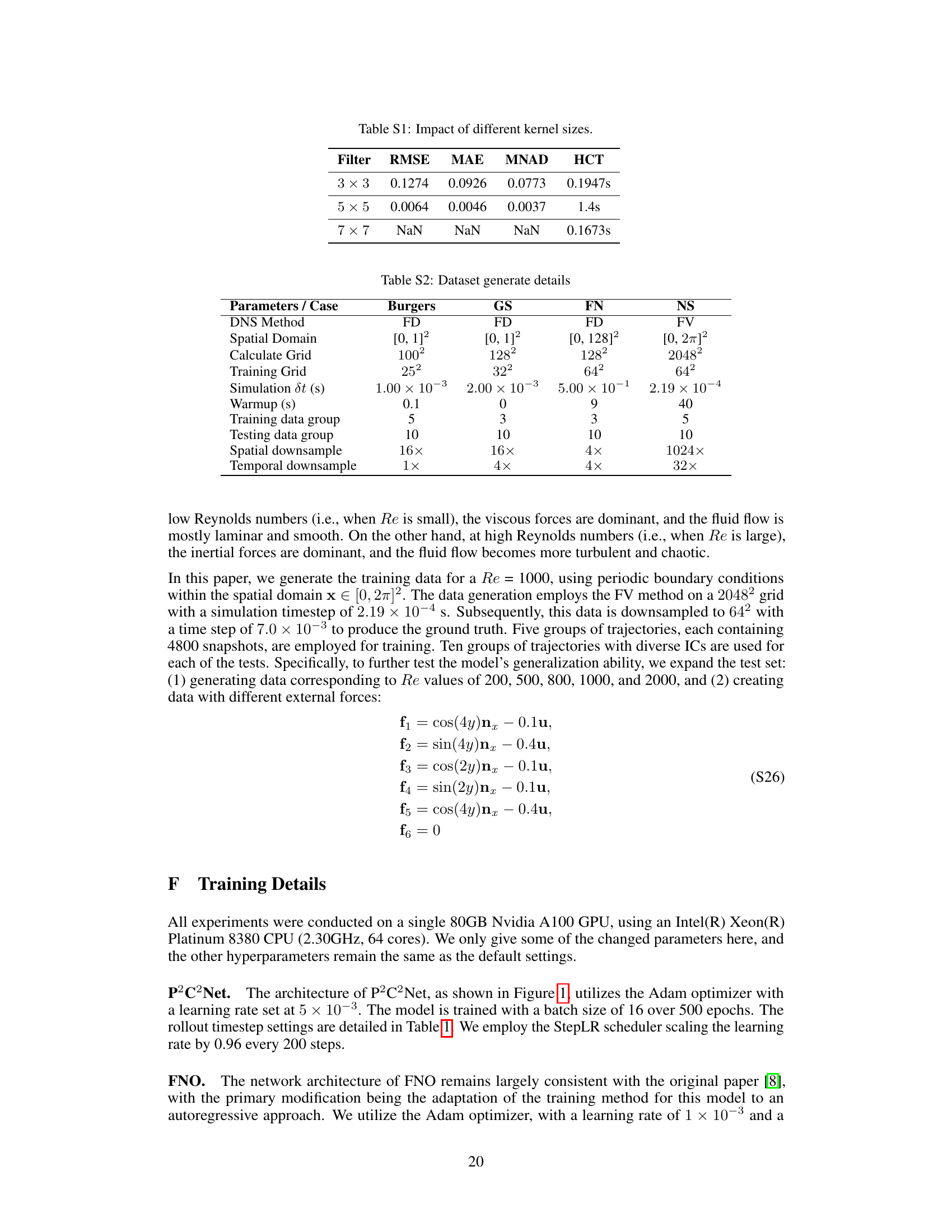
🔼 This table presents the ablation study results on the impact of different kernel sizes (3x3, 5x5, and 7x7) used in the learnable symmetric convolution filter within the P2C2Net model. The results are evaluated using four metrics: RMSE, MAE, MNAD, and HCT on the Burgers dataset. The 5x5 kernel shows significantly better performance compared to others, highlighting the impact of kernel size selection on the model’s accuracy and efficiency.
read the caption
Table S1: Impact of different kernel sizes.

🔼 This table summarizes the datasets used in the paper’s experiments, including the numerical methods used to generate the data (FD for finite difference, FV for finite volume), the spatial and temporal grid resolutions, the number of training and testing trajectories, and the number of rollout steps for each dataset. It also shows how the high-resolution simulation data was downsampled to create the lower-resolution training data used in the experiments. The table highlights the varying complexities of the datasets and training setups.
read the caption
Table 1: Summary of datasets and training implementations. Note that “→” denotes the downsampling process from the original resolution (simulation) to the low resolution (training).

🔼 This table shows the impact of adding Gaussian noise to the training data on the performance of the P2C2Net model. The results are presented in terms of RMSE, MAE, MNAD, and HCT. The table compares the performance metrics when 1% noise is added, when 0.5% noise is added, and when no noise is added.
read the caption
Table S3: Impact of noise on P2C2Net performance

🔼 This table presents the results of an ablation study conducted on the Burgers equation to evaluate the impact of reducing the training data size. It compares the model’s performance (RMSE, MAE, MNAD, and HCT) when trained with a reduced dataset (20% reduction) against the performance when trained with the original dataset (5 trajectories with 400 snapshots each). The results demonstrate the robustness of the P2C2Net model even with a significant reduction in training data.
read the caption
Table S4: Impact of sparser Burgers dataset on P2C2Net performance

🔼 This table presents a comparison of the P2C2Net model’s performance using two different types of boundary conditions: ‘Complex’ and ‘Periodic’. For each condition, the table shows the Root Mean Square Error (RMSE), Mean Absolute Error (MAE), Mean Normalized Absolute Difference (MNAD), and High Correction Time (HCT). The results demonstrate the model’s ability to generalize to different boundary conditions, achieving similar levels of accuracy in both cases.
read the caption
Table S5: Generalization of P2C2Net over different boundaries on the Burgers example for 10 trajectories.
Full paper#

