TL;DR#
Reinforcement Learning (RL) is powerful but can produce unsafe actions in critical systems due to its trial-and-error learning process. Existing safe RL methods either compromise safety or performance. This creates a need for algorithms that balance safety and performance.
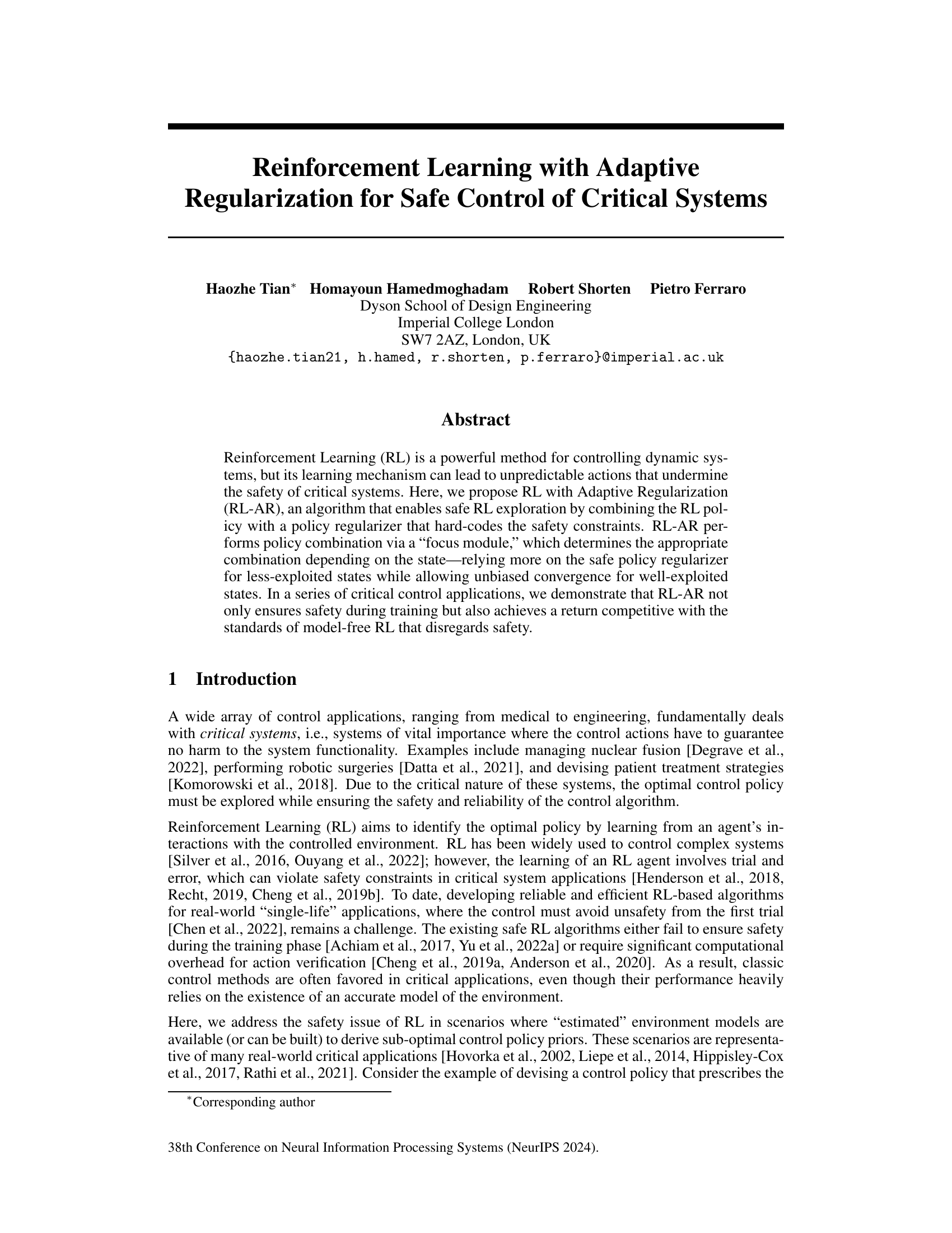
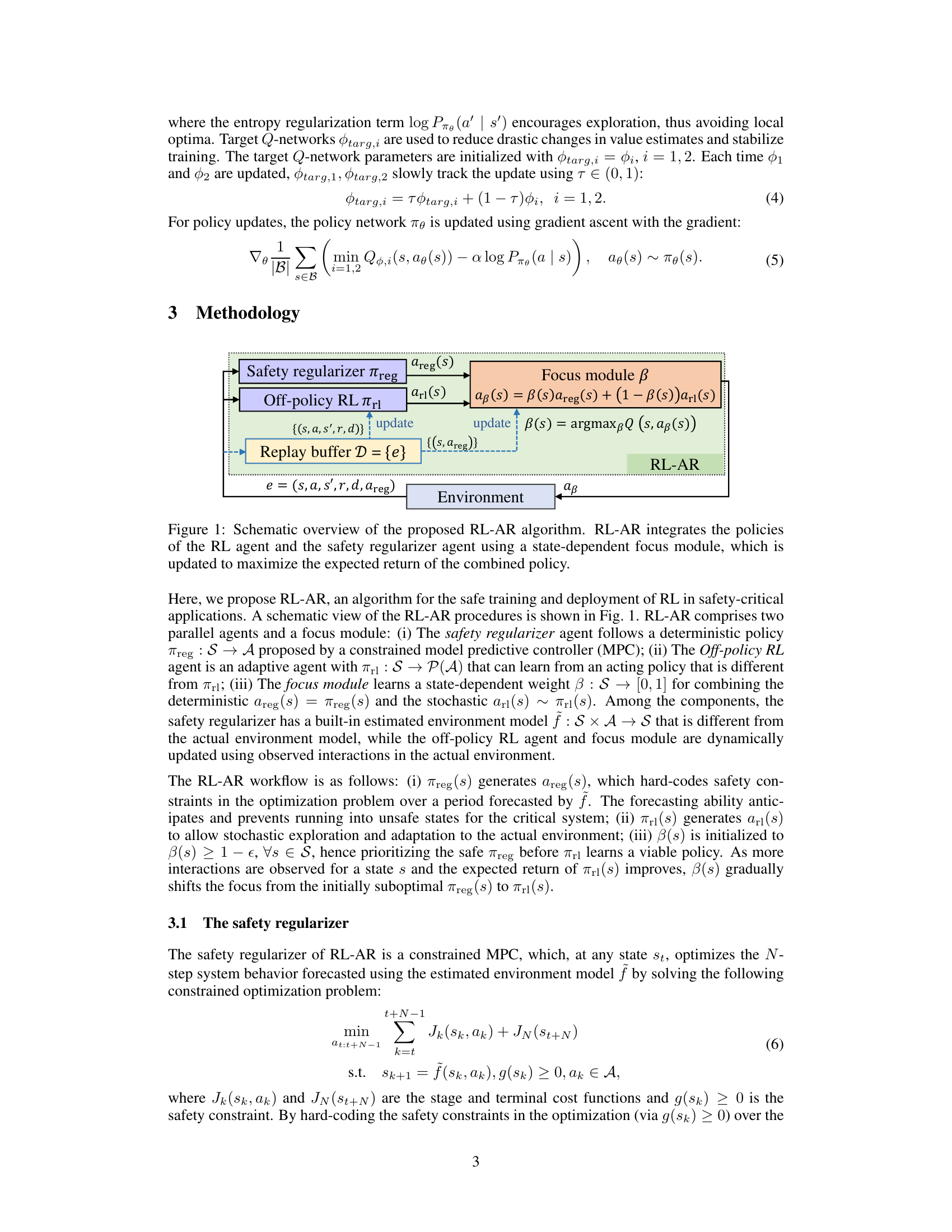
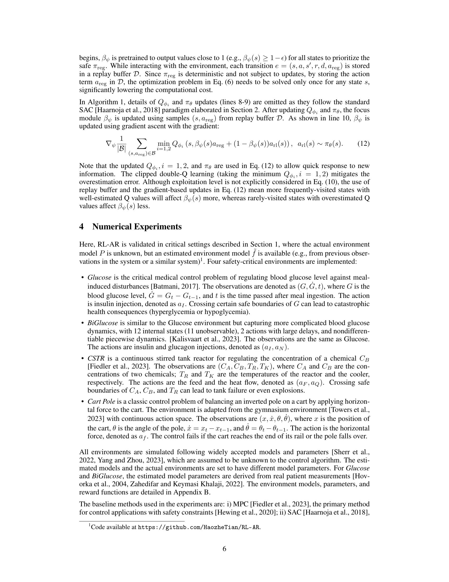
RL-AR, proposed in this paper, directly addresses this by integrating a safety regularizer with an RL agent. The safety regularizer avoids unsafe actions using an estimated environment model, while the RL agent learns from actual interactions. A focus module combines both agents’ policies based on the state’s exploration level. Results in critical control scenarios show that RL-AR ensures safety during training and outperforms existing methods in terms of return.
Key Takeaways#
Why does it matter?#
This paper is important because it presents RL-AR, a novel approach to safe reinforcement learning that is crucial for critical systems. It addresses the challenge of balancing exploration and exploitation while ensuring safety, offering a practical solution for real-world applications where safety is paramount. This work opens new avenues for research in safe RL, especially in areas with limited or uncertain models of the environment.
Visual Insights#

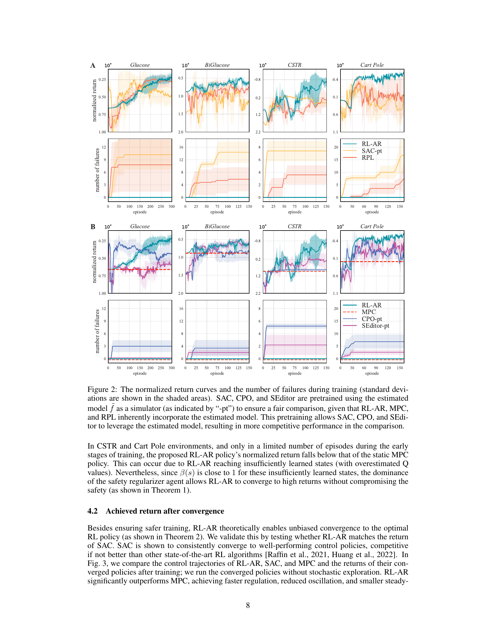
🔼 This figure compares the performance of RL-AR with other safe and unsafe RL algorithms across four different safety-critical control tasks. The top row shows the normalized episodic return for each algorithm over training episodes. The bottom row displays the cumulative number of training episodes that ended in failure for each algorithm. The results demonstrate that RL-AR consistently achieves higher returns while maintaining safety throughout the training process, in contrast to other methods that frequently experience failures, even with the benefit of pretraining using an estimated environment model.
read the caption
Figure 2: The normalized return curves and the number of failures during training (standard deviations are shown in the shaded areas). SAC, CPO, and SEditor are pretrained using the estimated model f as a simulator (as indicated by “-pt”) to ensure a fair comparison, given that RL-AR, MPC, and RPL inherently incorporate the estimated model. This pretraining allows SAC, CPO, and SEditor to leverage the estimated model, resulting in more competitive performance in the comparison.

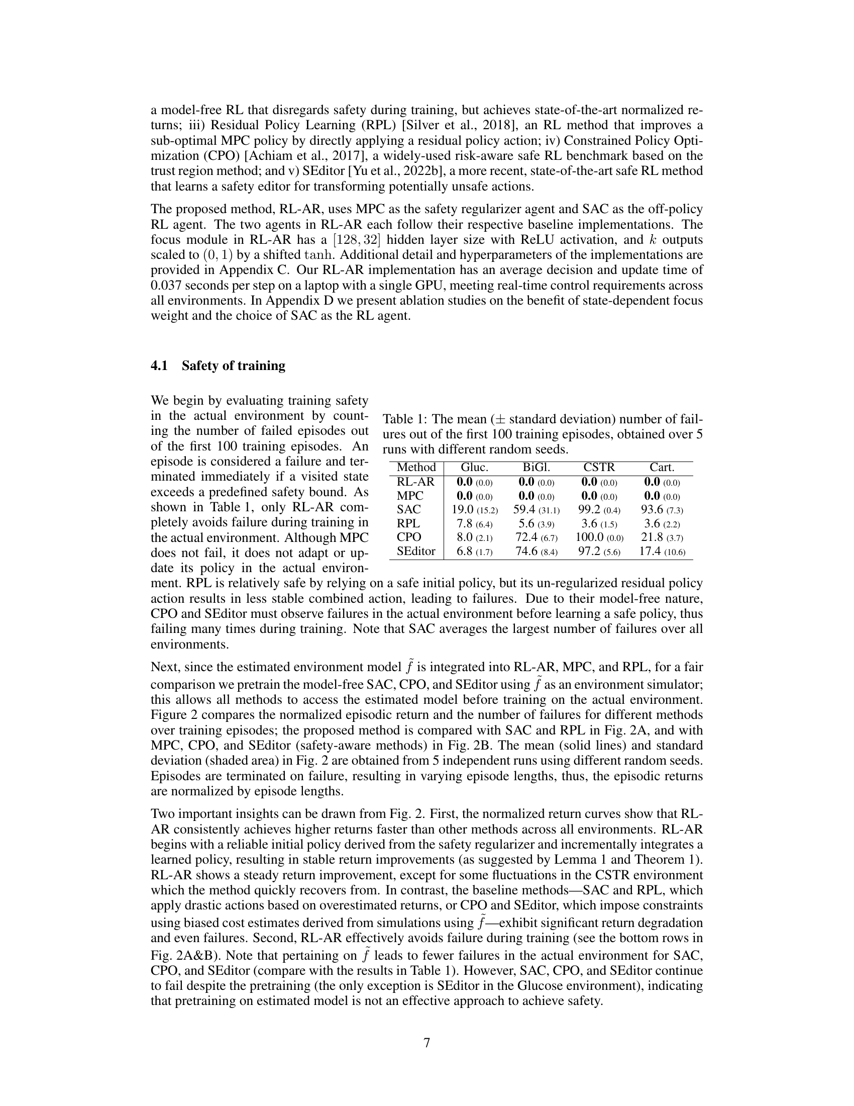
🔼 This table presents the number of failed training episodes for different RL algorithms in four safety-critical environments: Glucose, BiGlucose, CSTR, and Cart Pole. A failed episode is one where safety constraints are violated during training. The results show that only RL-AR successfully avoids failures during training, highlighting its safety and reliability compared to other methods.
read the caption
Table 1: The mean (± standard deviation) number of failures out of the first 100 training episodes, obtained over 5 runs with different random seeds.
In-depth insights#
Adaptive Regularization#
Adaptive regularization, in the context of reinforcement learning (RL) for critical systems, represents a crucial advancement in ensuring safety without significantly compromising performance. The core idea is to dynamically adjust the level of regularization applied to the RL agent’s policy based on the current state’s level of exploration. In less-explored states, where the risk of unsafe actions is higher, the algorithm heavily relies on a pre-defined safe policy (e.g., from a model predictive controller), effectively increasing the regularization. This prioritizes safety in uncertain regions. Conversely, in well-explored states, the algorithm reduces regularization, allowing the RL agent to learn and converge to an optimal policy unimpeded. This dynamic adjustment is often implemented via a ‘focus module’ that weighs the contributions of the safe and RL policies according to the state’s exploration level. This approach offers a powerful balance between safety and performance, addressing a long-standing challenge in applying RL to domains where mistakes are costly. The adaptive nature is key; it allows for safe initial deployment and a gradual shift towards optimal, yet safe, control as the agent’s understanding of the environment improves.
Safe RL Exploration#
Safe reinforcement learning (RL) exploration focuses on designing algorithms that guarantee safety during the learning process, a critical aspect when deploying RL in real-world applications with potential risks. A core challenge lies in balancing exploration (finding optimal policies) and exploitation (avoiding unsafe actions). Methods like adding safety constraints or using penalty functions can restrict exploration, potentially limiting the agent’s ability to find truly optimal solutions. Adaptive techniques, which modify the exploration strategy based on the agent’s current knowledge and risk assessment, are crucial. These could involve adjusting exploration parameters based on the proximity to unsafe states, using learned safety models to guide exploration, or employing a combination of safe and unsafe policies, switching between them according to context. Ensuring safety while maintaining sufficient exploration for good performance is a key research area; strategies vary, and finding the right balance often involves careful consideration of specific application contexts and risk tolerances. Theoretical analysis and rigorous empirical evaluation are vital for establishing the efficacy and limitations of any proposed safe exploration method.
Focus Module#
The focus module is a crucial component of the proposed RL-AR algorithm, acting as an arbiter between a risk-averse policy (safety regularizer) and a potentially unsafe but high-reward policy (off-policy RL agent). Its function is to dynamically combine these two policies according to the context, relying more on the safety policy in uncertain or unexplored states, and transitioning to the reward-focused policy as confidence in the learned model increases. This state-dependent weighting mechanism offers a unique approach to safe reinforcement learning, allowing for cautious exploration early in the learning process and gradually shifting towards riskier, potentially more rewarding behaviors as the agent’s knowledge improves. The effectiveness of this adaptive weighting is supported by both theoretical analysis, which demonstrates its role in regulating the effect of policy uncertainty, and empirical findings that confirm its contribution to achieving both safety and high rewards.
Safety-Critical Control#
Safety-critical control systems demand high reliability and dependability, as failures can have severe consequences. Traditional control methods often prioritize performance over safety, relying on accurate models and deterministic algorithms. However, these methods can be brittle and may not adapt well to unanticipated situations or model inaccuracies. Reinforcement learning (RL) offers the potential for adapting to complex, dynamic environments, but its inherent trial-and-error learning process can be unsafe for safety-critical applications. The challenge lies in designing RL algorithms that guarantee safety throughout the learning phase without sacrificing performance. Adaptive regularization techniques and constraint-based methods, such as those using Control Barrier Functions or Model Predictive Control, are crucial for developing safe and robust RL controllers. Verification and validation become paramount, needing robust methodologies to ensure that the learned policy consistently meets safety requirements. The research area requires a careful balance between leveraging RL’s adaptive capabilities and enforcing strict safety guarantees, necessitating a combination of theoretical analysis and extensive empirical testing.
Model Discrepancies#
The concept of ‘Model Discrepancies’ in reinforcement learning (RL) for critical systems is crucial. It acknowledges that real-world environments are complex and rarely perfectly captured by models. This imperfect modeling leads to discrepancies between the model’s predictions and the actual system behavior. The impact of these discrepancies is particularly significant in safety-critical applications where the consequences of errors can be catastrophic. A robust RL algorithm should be able to handle these discrepancies gracefully, ensuring safety and performance even when the model is inaccurate. The focus should be on strategies that either reduce the reliance on the model or incorporate mechanisms to adapt to model inaccuracies, such as robust optimization techniques, or a combination of model-based and model-free methods. Moreover, quantifying the level of acceptable model discrepancy to still guarantee safety is a critical challenge that demands careful consideration. This requires rigorous analysis and testing under various degrees of model mismatch.
More visual insights#
More on figures
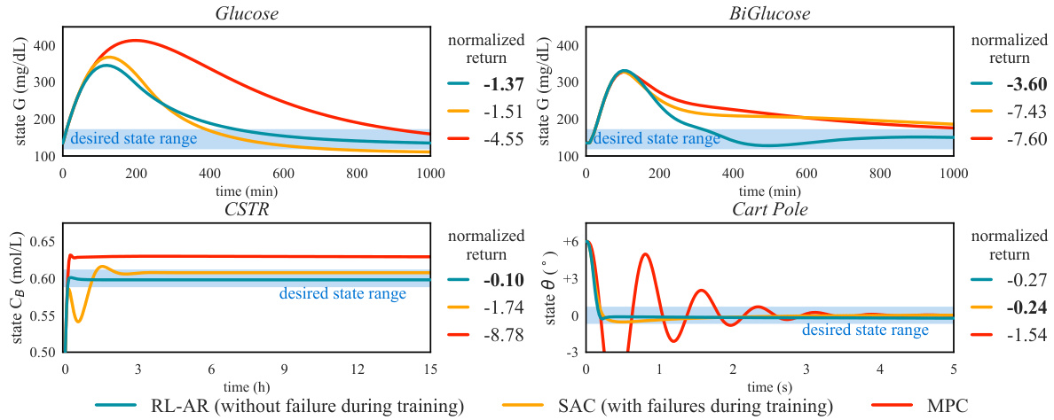
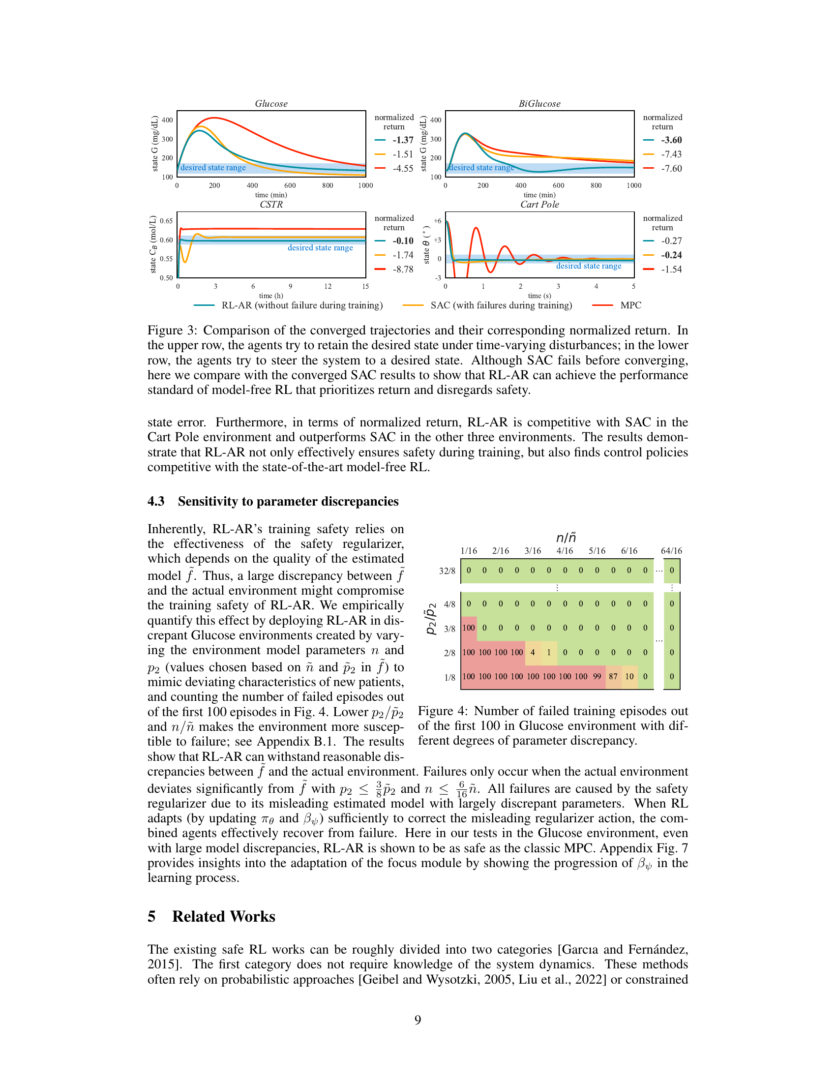
🔼 This figure compares the performance of RL-AR with SAC and MPC after both algorithms have converged. The top row shows scenarios where the agents attempt to maintain a desired state despite time-varying disturbances. The bottom row shows scenarios where the agents aim to move the system to a specific state. Despite SAC’s failures during training, the converged results demonstrate that RL-AR achieves the performance of model-free RL algorithms that prioritize reward over safety.
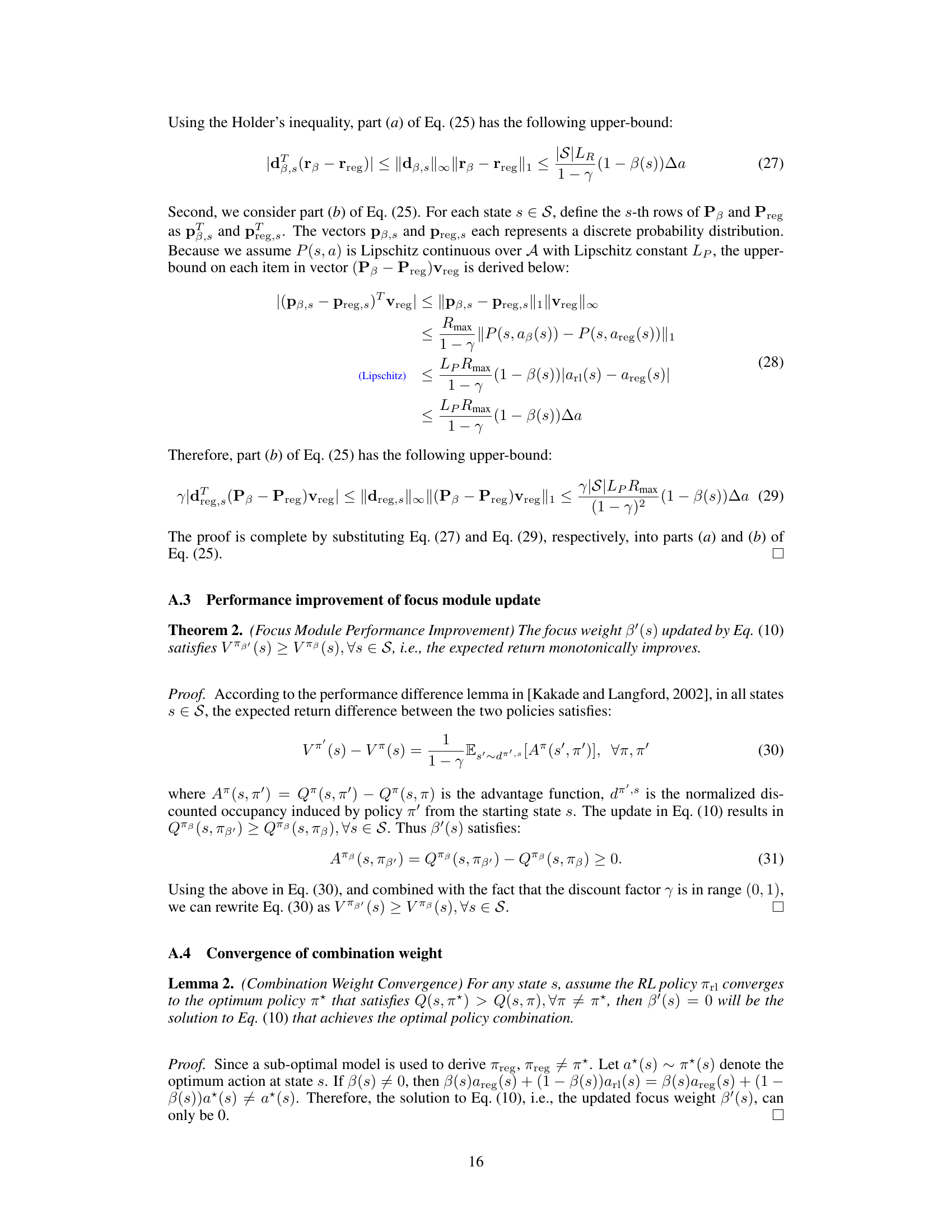
read the caption
Figure 3: Comparison of the converged trajectories and their corresponding normalized return. In the upper row, the agents try to retain the desired state under time-varying disturbances; in the lower row, the agents try to steer the system to a desired state. Although SAC fails before converging, here we compare with the converged SAC results to show that RL-AR can achieve the performance standard of model-free RL that prioritizes return and disregards safety.
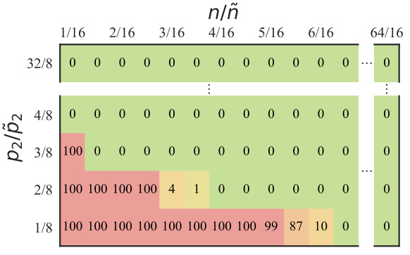
🔼 The figure shows the number of failed training episodes in the Glucose environment when varying the levels of discrepancies between the estimated model and the actual environment. The discrepancies are created by adjusting the parameters p2 and n to mimic the characteristics of new patients. The results demonstrate that RL-AR can withstand certain levels of discrepancies without compromising safety. Failures occur only when the actual environment deviates significantly from the estimated model.
read the caption
Figure 4: Number of failed training episodes out of the first 100 in Glucose environment with different degrees of parameter discrepancy.
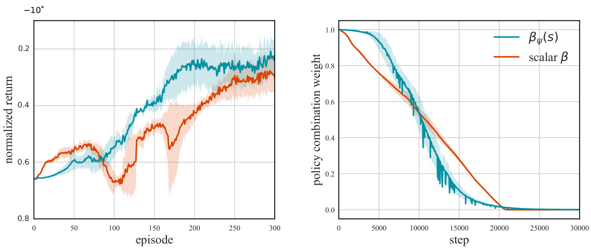
🔼 The figure compares the performance of RL-AR using a state-dependent focus module (βy(s)) against a scalar focus module (β). The left panel shows the normalized return curves for both approaches over training episodes, highlighting that state-dependent policy combination leads to more stable returns compared to a fixed scalar value. The right panel displays the evolution of the focus weights over training steps. Both methods converge towards 0, but the state-dependent version exhibits fluctuations due to its adaptive nature, dynamically adjusting the policy combination based on state-specific needs.
read the caption
Figure 5: Comparing the state-dependent focus module βy(s) with the scalar β by plotting the normalized return curves (left) and focus weight curves (right) in the Glucose environment. Shaded areas indicate standard deviations.

🔼 The figure compares the performance of RL-AR using SAC and TD3 as the reinforcement learning module in the Glucose environment. The key difference between SAC and TD3 is the entropy regularization term in SAC, which promotes exploration and stability. The plot shows normalized return over training episodes. SAC consistently outperforms TD3, highlighting the benefits of entropy regularization in this specific environment.
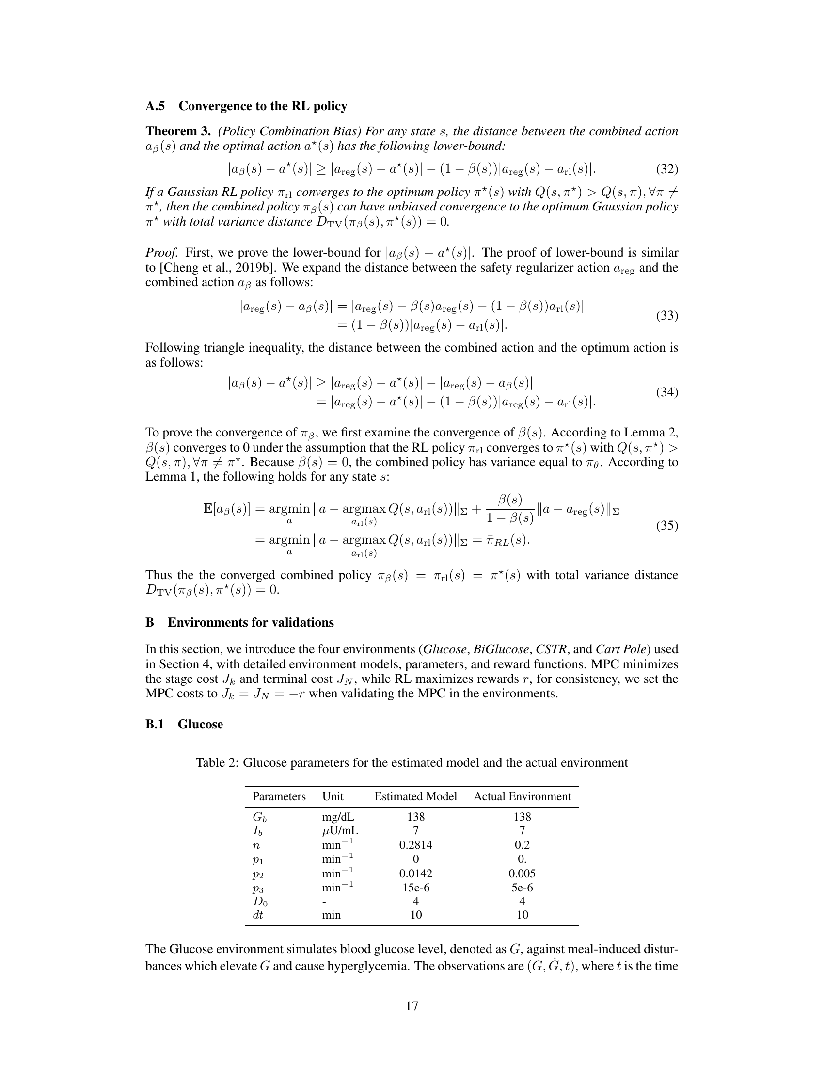
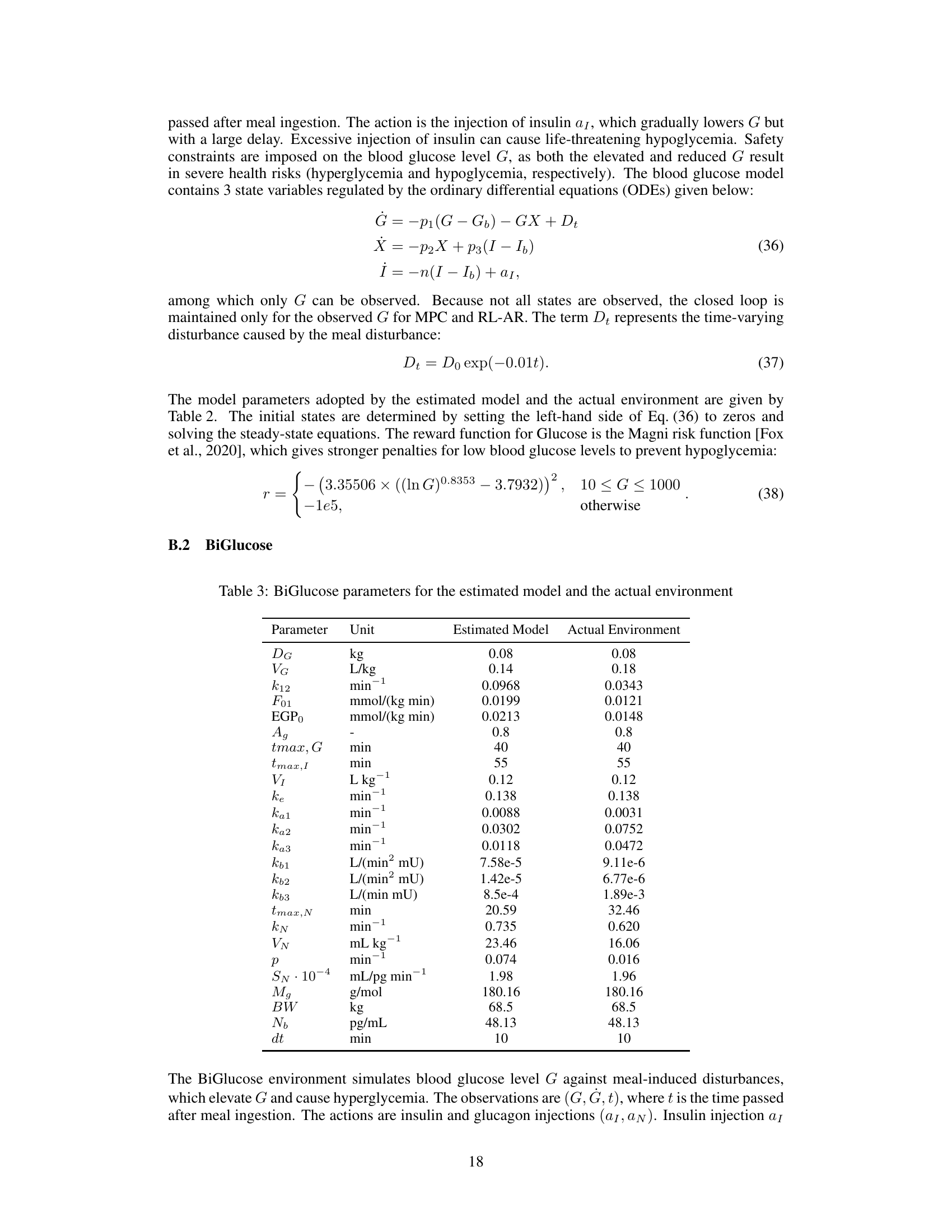
read the caption
Figure 6: Comparison of normalized return between using the SAC and using TD3 [Fujimoto et al., 2018] as the RL agent in the Glucose environment (standard deviations are shown in the shaded area). The main difference between SAC and TD3 is that SAC has the entropy regularization terms in its objectives, which are intended to encourage diverse policies and stabilize training.
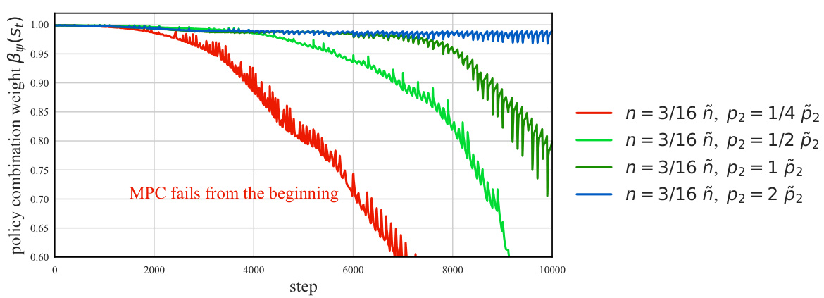
🔼 This figure shows the evolution of the focus weights (β(s)) during training of RL-AR in various Glucose environments with different levels of discrepancies between the estimated and actual environment models. The x-axis represents the training steps, and the y-axis represents the focus weight. Each line represents a different level of discrepancy, with each color representing different parameters (p2, n). The figure shows how the focus weight adapts to the discrepancies. When there is a large discrepancy, the focus weight decreases rapidly, enabling RL-AR to recover from initial failures. Conversely, when the discrepancy is smaller, the focus weight converges more slowly. The plot shows how the proposed RL-AR method adapts the policy combination (focus) based on the actual environment experience. It showcases the resilience of the method to parameter mismatches, highlighting its adaptability and reliability in real-world scenarios.
read the caption
Figure 7: The focus weights when training with varying levels of discrepancies between the estimated Glucose model (with parameters p2, ñ) and the actual Glucose environment (with parameters P2, n).

🔼 This figure shows the training performance of RL-AR, MPC, and SAC (pretrained) on the Acrobot environment. The left panel displays the normalized return achieved by each algorithm over a series of training episodes. RL-AR demonstrates a consistently higher and more stable return compared to the others, particularly exceeding SAC (pretrained) in the long run. The right panel shows the cumulative number of failures (episodes ending prematurely due to unsafe states). RL-AR achieves near-zero failures, highlighting its safety benefits during training, unlike SAC (pretrained) which experiences many failures, and MPC which consistently fails from the beginning. The results reinforce RL-AR’s ability to achieve better performance while maintaining safety compared to model-free methods (like SAC) and model-based methods (like MPC).
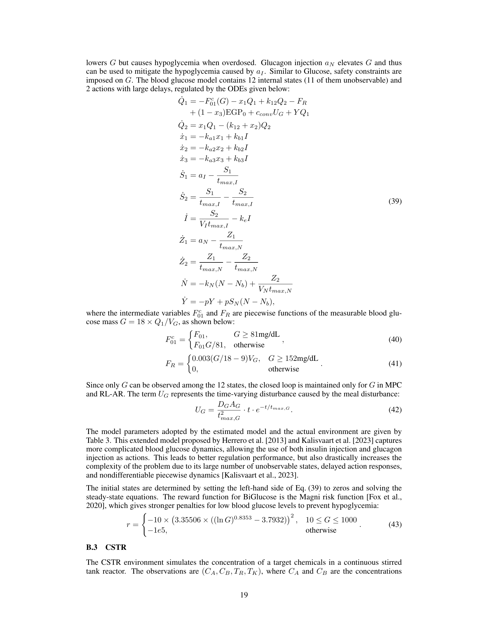
read the caption
Figure 8: Normalized return (left) and the number of failures (right) during training in the Acrobot environment (standard deviations are shown in the shaded area).
More on tables

🔼 This table presents the number of training failures for each RL algorithm across four different environments. A failure is defined as an episode where a safety constraint is violated. The numbers represent the average number of failures and standard deviation across five independent runs, each initiated with different random seeds. The data is intended to show the safety of the algorithms during training.
read the caption
Table 1: The mean (± standard deviation) number of failures out of the first 100 training episodes, obtained over 5 runs with different random seeds.

🔼 This table presents the parameters used in the glucose model for both the estimated model and the actual environment. It lists the values for parameters such as baseline glucose level (Gb), baseline insulin level (Ib), glucose decay rate (n), glucose absorption rates (p1, p2, p3), meal disturbance magnitude (Do), and the time step (dt). The differences between the estimated and actual parameter values represent the discrepancies between the model and the real-world system, which are crucial for testing the robustness of the proposed RL-AR algorithm.
read the caption
Table 2: Glucose parameters for the estimated model and the actual environment
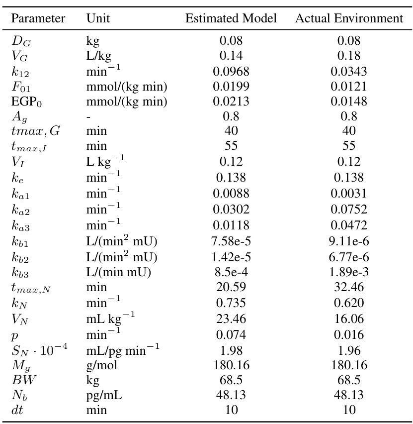
🔼 This table presents the parameters used in the BiGlucose model, comparing the values used in the estimated model and the actual environment. These parameters are crucial for simulating the blood glucose dynamics in this model, as differences between the estimated model and the actual environment introduce discrepancies that the RL-AR algorithm must handle.
read the caption
Table 3: BiGlucose parameters for the estimated model and the actual environment

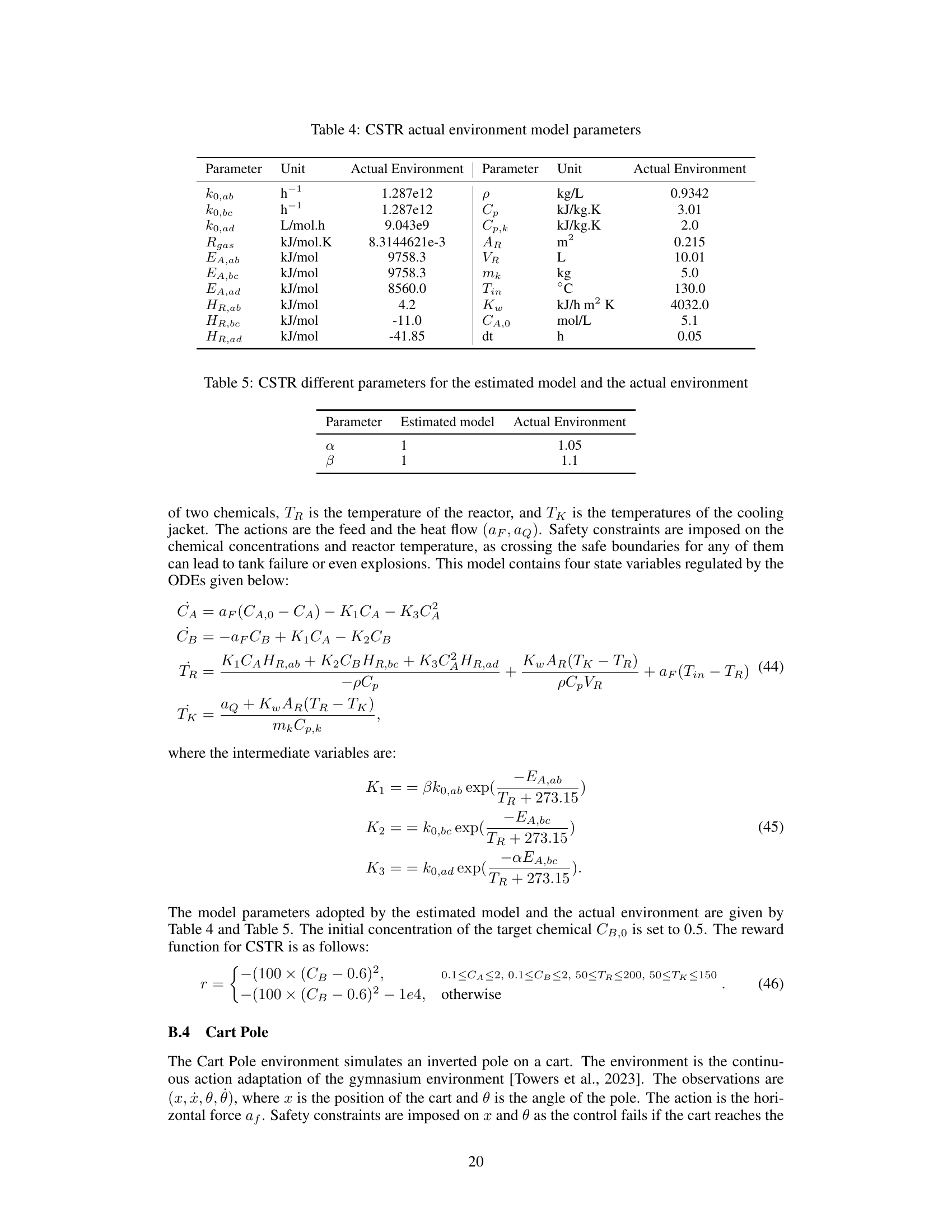
🔼 This table presents the parameters used to model the Continuous Stirred Tank Reactor (CSTR) system in the actual environment. These parameters define the kinetic and thermodynamic properties of the chemical reactions taking place within the reactor, as well as the physical properties of the reactor itself. These values are crucial for accurately simulating the CSTR’s behavior and are used in the equations governing the concentrations of the two chemicals (CA and CB), the reactor temperature (TR), and the temperature of the cooling jacket (TK).
read the caption
Table 4: CSTR actual environment model parameters

🔼 This table shows the parameters used in the CSTR (Continuous Stirred Tank Reactor) simulation. It lists the values for two parameters, α and β, in both an estimated model and the actual environment. These parameters are likely related to the reactor dynamics and their differences could indicate model inaccuracies or uncertainties impacting controller performance. This table supports the section on numerical experiments where this environment is used to validate the RL-AR algorithm, showcasing its performance under differing model/environment parameters.
read the caption
Table 5: CSTR different parameters for the estimated model and the actual environment

🔼 This table lists the parameters used in the Cart Pole environment simulation. It shows a comparison between the parameters used in the estimated model (used for training the safety regularizer) and the actual environment model. The parameters include gravitational acceleration (g), cart mass (mc), pole mass (mp), pole length (l), and the time step (dt). The discrepancies between the estimated and actual parameters highlight the challenge of safe reinforcement learning in real-world settings, where perfect model knowledge is rarely available.
read the caption
Table 6: Cart Pole parameters for the estimated model and the actual environment
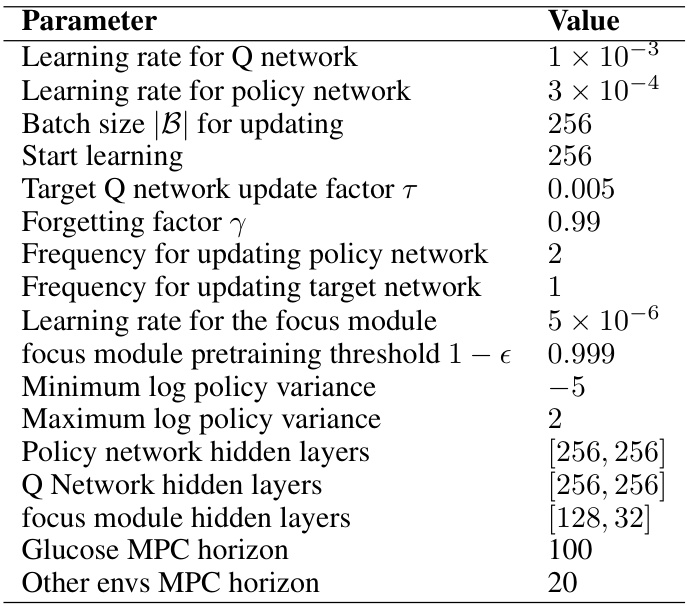
🔼 This table lists the hyperparameters used for the RL-AR algorithm. It shows the learning rates for the Q-network and policy network, the batch size for updating, the start learning step, the target Q-network update factor, the forgetting factor, the frequencies for updating the policy network and target network, the learning rate for the focus module, the focus module pretraining threshold, the minimum and maximum log policy variance, and the number of hidden layers in the policy network, Q-network and focus module. Finally, it shows the MPC horizon used for the Glucose environment and other environments. The baseline methods used the same network structures and training hyperparameters.
read the caption
Table 7: RL-AR hyperparameters. The baseline methods utilized the same network structures and training hyperparameters.
Full paper#
