↗ arXiv ↗ Hugging Face ↗ Hugging Face ↗ Chat
TL;DR#
Generating high-quality samples from cutting-edge diffusion models often necessitates computationally expensive numerical integration. Rectified flows offer an iterative approach, learning smooth ODE paths to mitigate truncation errors, but still require many function evaluations. This poses a challenge in competing with the efficiency of knowledge distillation methods.
This research introduces several novel training strategies for rectified flows to solve this problem. By observing that under realistic settings, a single Reflow iteration is sufficient to learn almost straight trajectories, the researchers optimize the single-iteration training process using a U-shaped timestep distribution and LPIPS-Huber premetric. This leads to remarkable improvements in the Fréchet Inception Distance (FID) score, outperforming existing distillation methods like consistency distillation and progressive distillation in low-NFE scenarios.
Key Takeaways#
Why does it matter?#
This paper is important because it significantly improves the training of rectified flows, a promising method for generating high-quality samples from diffusion models. The improved training techniques make rectified flows competitive with knowledge distillation methods, even with a low number of function evaluations. This addresses a key limitation of rectified flows and opens new avenues for research in efficient sampling from generative models. The work’s focus on practical training improvements, rather than theoretical advancements, is of significant value to applied researchers.
Visual Insights#
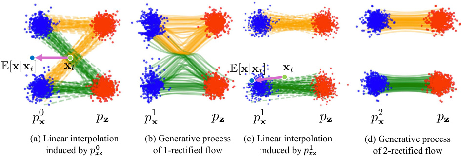
🔼 This figure illustrates the rectified flow process, showing how it iteratively learns smooth ODE paths to reduce truncation error. Panel (a) shows linear interpolation between two distributions (px and pz). Panel (b) shows how rectified flow transforms these paths to eliminate intersections. Panels (c) and (d) demonstrate the iterative refinement of these trajectories through the Reflow algorithm, resulting in straighter, less error-prone paths.
read the caption
Figure 1: Rectified flow process (figure modified from Liu et al. [2022]). Rectified flow rewires trajectories so there are no intersecting trajectories (a) → (b). Then, we take noise samples from pz and their generated samples from px, and linearly interpolate them (c). In Reflow, rectified flow is applied again (c) → (d) to straighten flows. This procedure is repeated recursively.

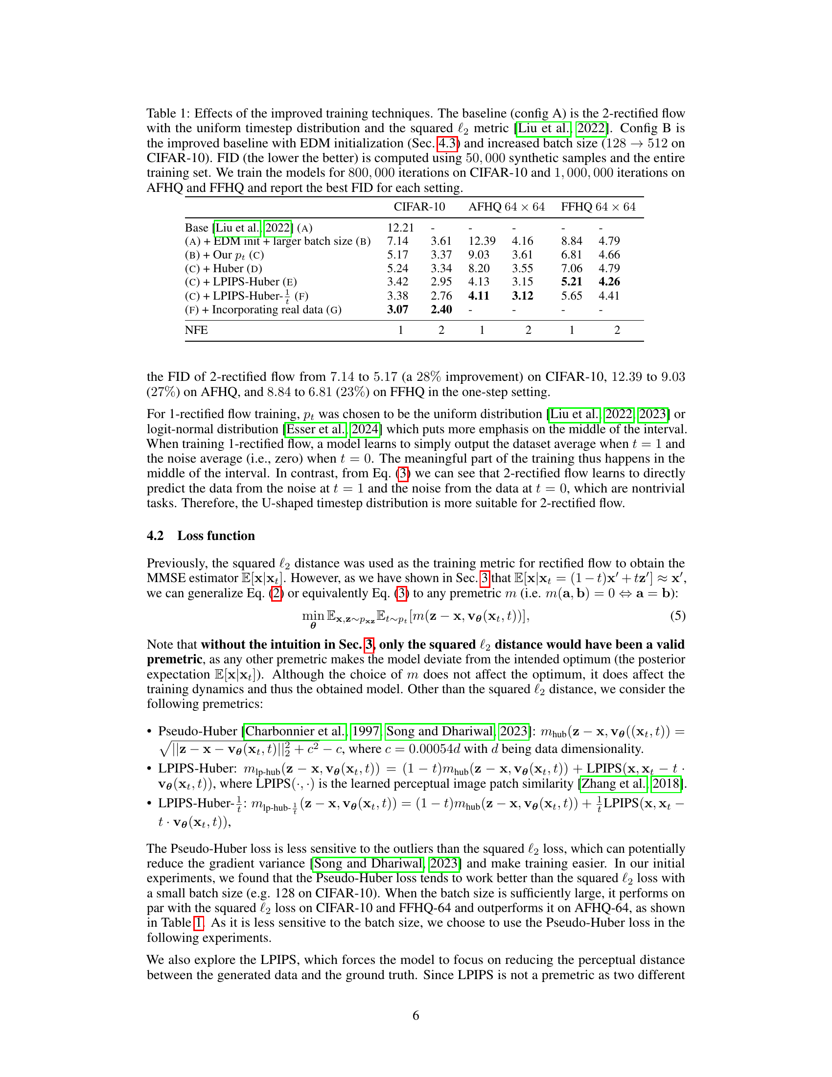
🔼 This table presents the results of an ablation study comparing different training techniques for 2-rectified flows. It shows how various configurations impact the Fréchet Inception Distance (FID) score, a metric for evaluating the quality of generated images. The configurations involve changes to the timestep distribution, loss function, model initialization, and incorporation of real data.
read the caption
Table 1: Effects of the improved training techniques. The baseline (config A) is the 2-rectified flow with the uniform timestep distribution and the squared l2 metric [Liu et al., 2022]. Config B is the improved baseline with EDM initialization (Sec. 4.3) and increased batch size (128 → 512 on CIFAR-10). FID (the lower the better) is computed using 50,000 synthetic samples and the entire training set. We train the models for 800,000 iterations on CIFAR-10 and 1,000,000 iterations on AFHQ and FFHQ and report the best FID for each setting.
In-depth insights#
Reflow Algorithm#
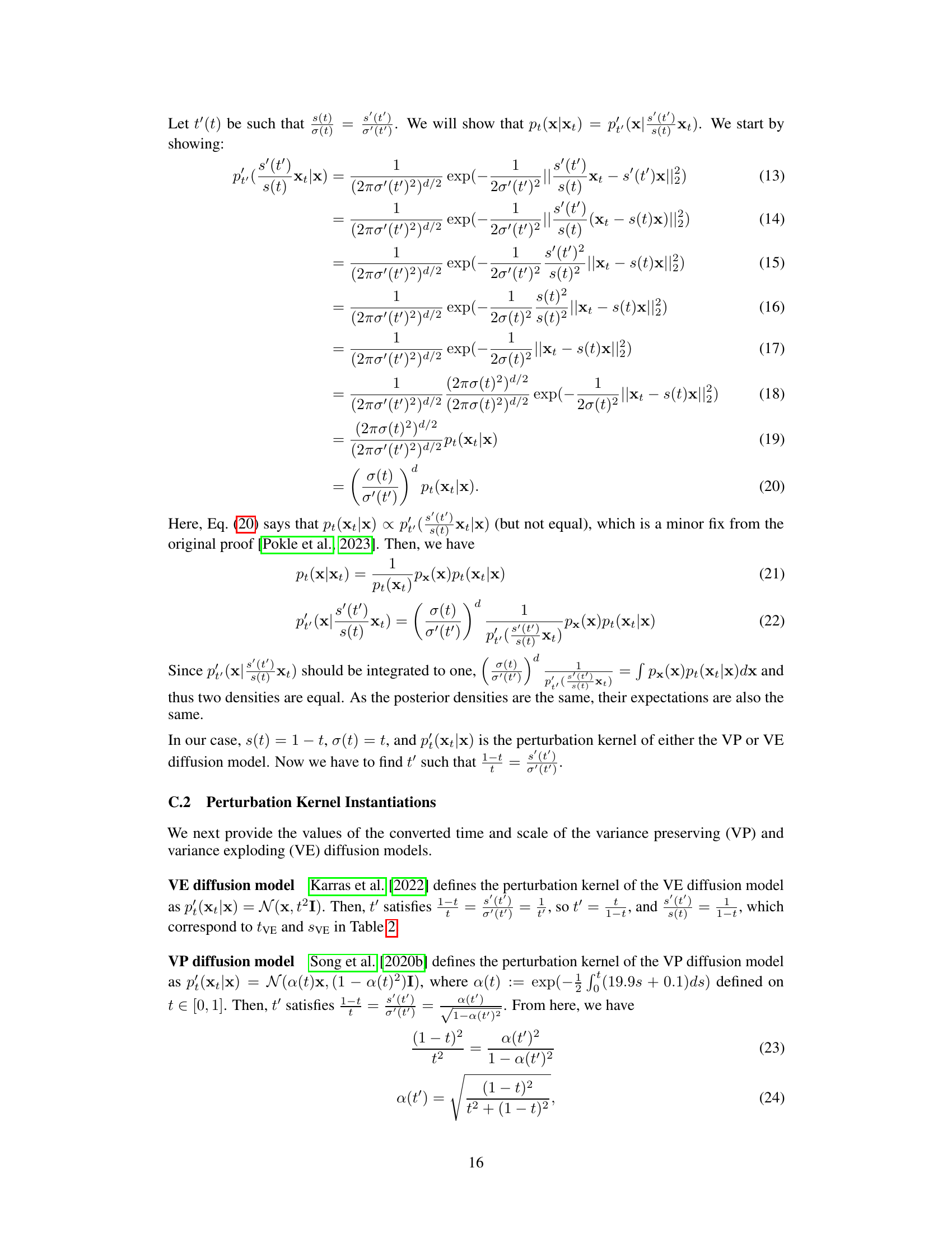
The Reflow algorithm, a recursive training procedure for rectified flows, aims to improve the quality of generated samples by iteratively refining the learned ODE trajectories. Its core idea is to leverage the generative ODE of a previously trained rectified flow to generate synthetic data-noise pairs. These pairs are then used to train a new rectified flow, leading to increasingly straighter trajectories. While effective, Reflow’s recursive nature can be computationally expensive, requiring multiple iterations and substantial resources for each stage. Each iteration involves generating data-noise pairs and training a model until convergence. This iterative process accumulates errors across rounds, potentially impacting the overall performance of the final model. The paper’s key contribution lies in demonstrating that, under realistic settings, a single iteration of Reflow may suffice. This significantly reduces computational costs, making rectified flows more competitive with distillation methods in low-NFE settings.
Training Refinements#
The effectiveness of rectified flows hinges significantly on training methodologies. The paper explores several key training refinements to boost performance, particularly in the low NFE regime. A U-shaped timestep distribution proves crucial; unlike uniform distributions, it prioritizes training on more challenging timesteps. This approach, combined with a shift to the LPIPS-Huber loss function, further enhances performance by focusing the model on perceptually meaningful discrepancies rather than simply pixel-level differences. The initialization method is also refined, leveraging pre-trained diffusion models to accelerate the process and enhance the quality of the resulting flows. By iteratively refining these aspects of the training process, the researchers demonstrate substantial improvements in FID scores, marking a significant step towards achieving competitive results with knowledge distillation methods while significantly reducing computational cost.
Low-NFE Competitiveness#
The concept of ‘Low-NFE Competitiveness’ in the context of generative models, specifically rectified flows, centers on achieving high-quality sample generation with a minimal number of function evaluations (NFEs). This is crucial for computational efficiency. The paper likely highlights how rectified flows, despite their inherent advantage of generating smooth ODE paths reducing truncation errors, still require more NFEs than knowledge distillation methods. A key contribution would be demonstrating that with improved training techniques (e.g., U-shaped timestep distribution, LPIPS-Huber premetric), rectified flows can match or even surpass the performance of distillation methods, even in the low-NFE regime. This is a significant advancement, making rectified flows a more practical and computationally feasible alternative. The analysis likely explores the reasons behind the success of these training improvements, possibly by showing that under realistic settings, a single iteration of the Reflow algorithm suffices for learning near-straight trajectories, making multiple iterations redundant. Achieving competitiveness in the low-NFE setting is valuable because it directly addresses a critical limitation of diffusion models, and it showcases the versatility and potential of rectified flows in real-world applications where efficiency is paramount. The paper likely presents this competitiveness through empirical results, showing improved FID scores compared to other state-of-the-art techniques across multiple datasets and various NFE settings.
Inversion Applications#
The concept of “Inversion Applications” in the context of diffusion models and rectified flows is significant because it highlights the unique ability of these models to reverse the generative process, mapping generated data back to the original latent space. Unlike many other generative models, this inversion capability isn’t simply a byproduct; it’s a core functionality with many downstream applications. Image editing becomes significantly easier, allowing for precise manipulations and control over the generated content. High-quality image editing is often difficult with other methods due to the lack of understanding of the underlying latent space. In the same vein, image-to-image translation becomes more natural using this inversion technique; the process of transforming one image into another is significantly easier and more accurate by first mapping both images into the same latent space, and then transforming the desired image using the rectified flows. Furthermore, this inversion ability opens doors to other applications, such as watermarking and data-to-noise transformations, improving security and other unique creative applications.
Future Work#
Future research directions stemming from this work on rectified flows could involve exploring alternative architectures to enhance the model’s efficiency and scalability. Investigating novel loss functions beyond LPIPS-Huber, perhaps incorporating adversarial training techniques, could further refine the model’s ability to learn high-quality, low-NFE samples. A promising avenue would be to systematically investigate different ODE solvers and their impact on the overall performance and computational cost. Exploring more advanced sampling strategies is also crucial. Finally, exploring the application of rectified flows to other generative modeling tasks beyond image synthesis, such as video generation or other modalities, presents exciting possibilities. A comprehensive investigation into the model’s limitations, particularly its computational cost in higher-NFE scenarios and its sensitivity to hyperparameters, would enable a deeper understanding of the underlying mechanisms and help to build more robust and efficient rectified flow models.
More visual insights#
More on figures
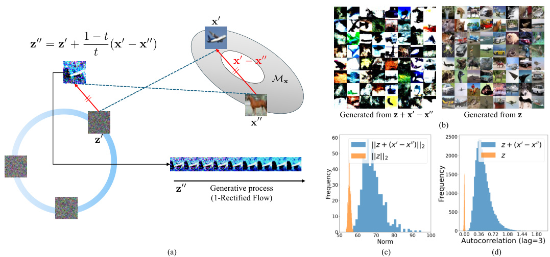
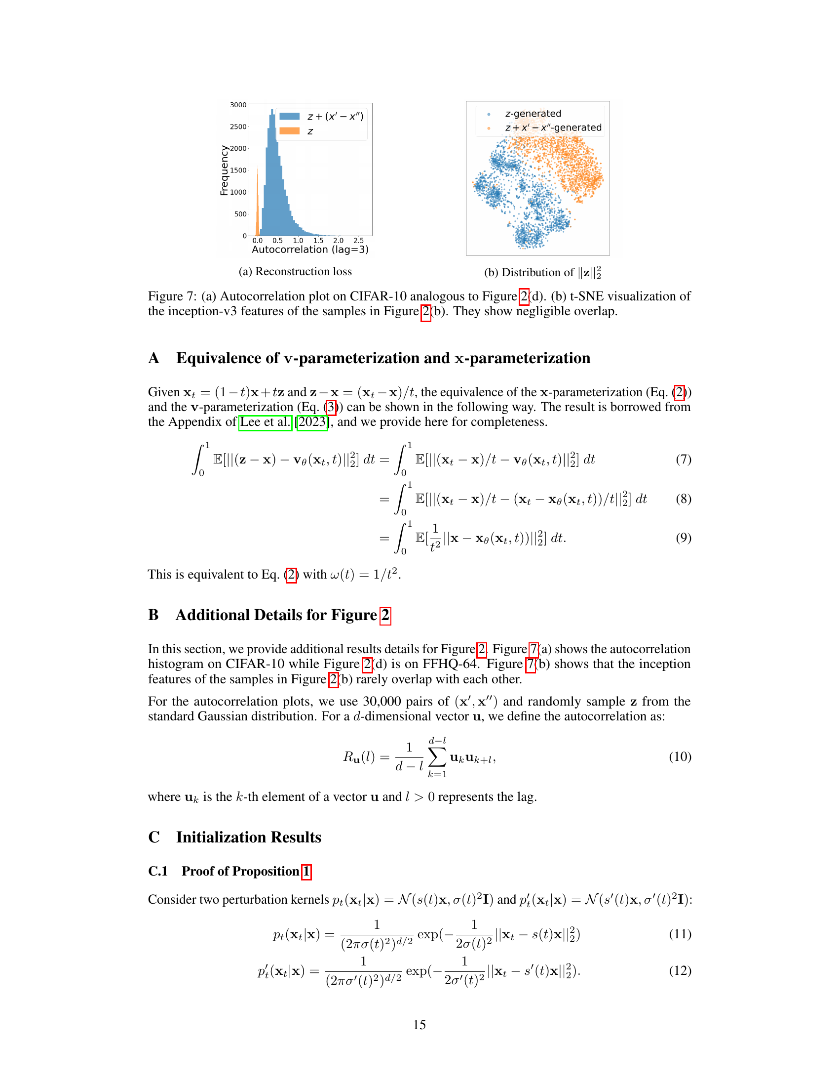
🔼 This figure illustrates the intuition behind applying Reflow only once. It shows that if linear interpolation trajectories intersect (meaning the generated noise z is not typical), the 1-rectified flow struggles to map it back to the data space. This suggests that under realistic data distributions, multiple Reflow iterations are unnecessary because the trajectories are already approximately straight after one iteration. The figure supports this by showing that (a) intersecting trajectories lead to atypical noise samples, (b) directly using atypical noise in generating samples produces poor results, (c) atypical noise samples have unusually high norms, and (d) atypical noise samples exhibit high autocorrelation, unlike typical Gaussian noise.
read the caption
Figure 2: An illustration of the intuition in Sec. 3. (a) If two linear interpolation trajectories intersect, z' - z' is parallel to x' – x'. This generally maps z' to an atypical (e.g., one with high autocorrelation or a norm that is too large to be on a Gaussian annulus) realization of Gaussian noise, so the 1-rectified flow cannot reliably map z' to x' on Mx. (b) Generated samples from the pre-trained 1-rectified flow starting from z ~ N(0, I) (right), which is the standard setting, and z' = z + (x' – x'), where x', x' are sampled from 1-rectified flow trained on CIFAR-10 (left). Qualitatively, we see that the left samples have very low quality. (c) Empirically, we show the l2 norm of z' = z + (x' – x') compared to z', which is sampled from the standard Gaussian. z' generally lands outside the annulus of typical Gaussian noise. (d) z + (x' – x') has high autocorrelation while the autocorrelation of Gaussian noise is nearly zero in high-dimensional space.
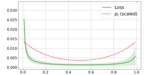
🔼 This figure shows the training loss curve for a vanilla 2-rectified flow model on the CIFAR-10 dataset. The x-axis represents the timestep, and the y-axis represents the training loss. The shaded region shows the standard deviation of the loss across multiple runs. A U-shaped curve is overlaid on the plot, which represents the proposed timestep distribution for training the model; it is scaled for better visualization. The plot demonstrates that the loss is higher at the beginning and end of the timestep range and lower in the middle, supporting the U-shaped timestep distribution used in the improved training method.
read the caption
Figure 3: Training loss of the vanilla 2-rectified flow on CIFAR-10 measured on 5,000 samples after 200,000 iterations. The shaded area represents the 1 standard deviation of the loss. The dashed curve is our U-shaped timestep distribution, scaled by a constant factor for visualization.

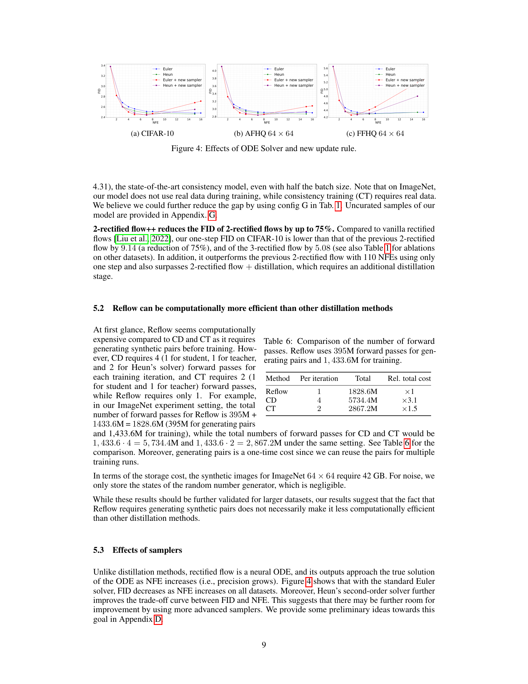
🔼 This figure shows the effects of different ODE solvers (Euler and Heun) and a new update rule on the FID (Frechet Inception Distance) for three different datasets: CIFAR-10, AFHQ 64x64, and FFHQ 64x64. The x-axis represents the number of function evaluations (NFEs), and the y-axis represents the FID. Lower FID values indicate better image quality. The figure demonstrates that the new update rule significantly improves sampling efficiency across all datasets and solvers, achieving the best FID with fewer NFEs. The plots highlight the trade-off between FID and NFE. Generally, Heun’s method outperforms the Euler method.
read the caption
Figure 4: Effects of ODE Solver and new update rule.

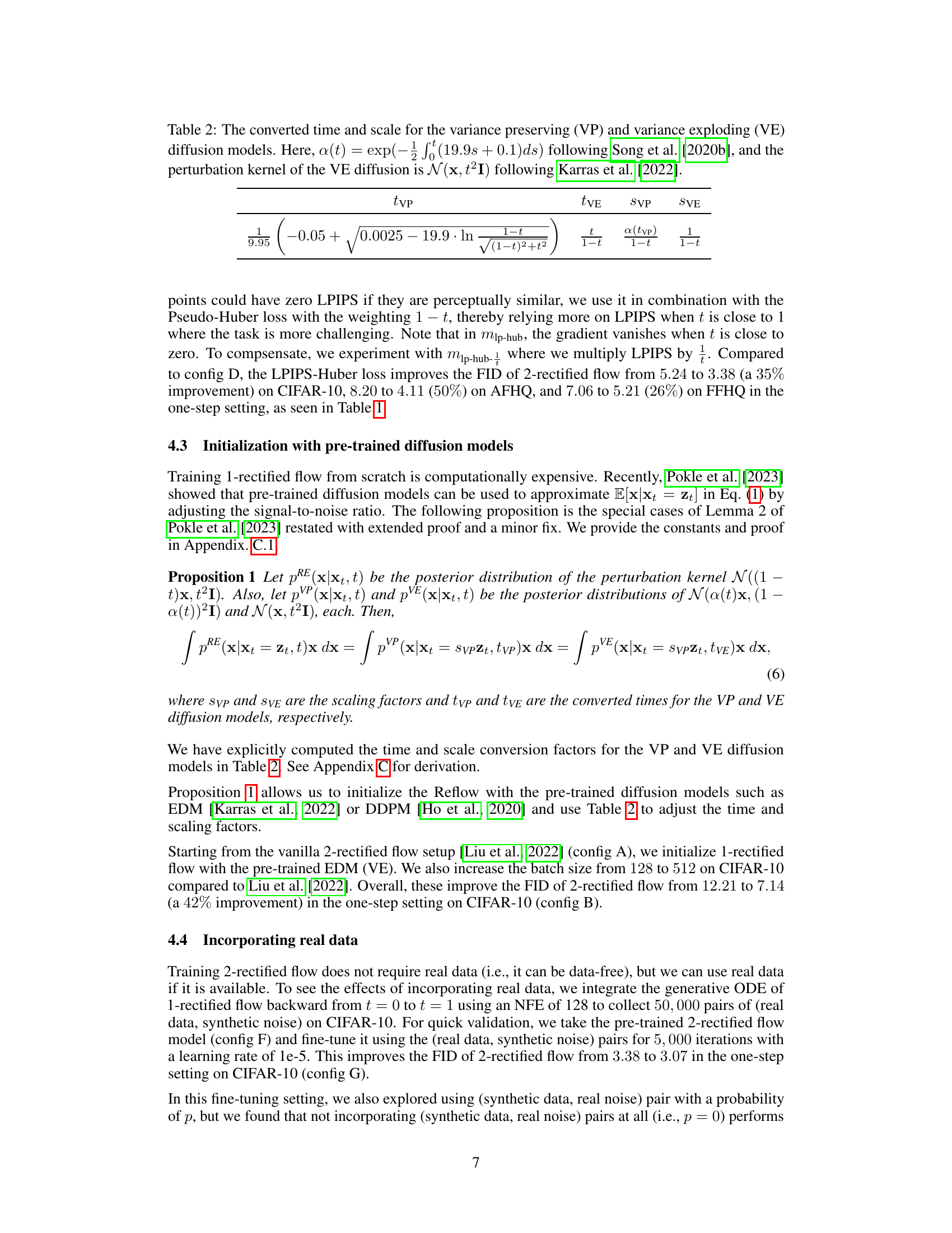
🔼 This figure demonstrates the inversion capabilities of the proposed 2-rectified flow++ model on CIFAR-10 dataset. It compares the reconstruction error with EDM, shows the distribution of the norm of inverted noise, and visually presents inversion and reconstruction results. The results highlight that 2-rectified flow++ achieves lower reconstruction error and more realistic noise compared to EDM, especially with fewer function evaluations.
read the caption
Figure 5: Inversion results on CIFAR-10. (a) Reconstruction error between real and reconstructed data is measured by the mean squared error (MSE), where the x-axis represents NFEs used for inversion and reconstruction (e.g., 2 means 2 for inversion and 2 for reconstruction). (b) Distribution of ||z||2 of the inverted noises as a proxy for Gaussianity (NFE = 8). The green histogram represents the distribution of true noise, which is Chi-squared with 3 × 32 × 32 = 3072 degrees of freedom. (c) Inversion and reconstruction results using (8 + 8) NFEs. With only 8 NFEs, EDM fails to produce realistic noise, and also the reconstructed samples are blurry.

🔼 This figure demonstrates two applications of few-step inversion using rectified flow. The first row shows the interpolation between two real images (dog and lion). The second row shows the image-to-image translation between two real images (tiger and lion). The total number of function evaluations (NFEs) used in each application is 6, where 4 NFEs are used for inversion and 2 NFEs are used for generation.
read the caption
Figure 6: Applications of few-step inversion. (a) Interpolation between two real images. (b) Image-to-image translation. The total NFEs used are 6 (4 for inversion and 2 for generation).

🔼 This figure illustrates the intuition behind applying Reflow only once. Panel (a) shows that if trajectories intersect, the resulting noise z’’ is atypical (high autocorrelation, large norm). Panel (b) shows that generating samples from this atypical noise leads to poor quality samples. Panel (c) shows that the norm of z’’ is larger than the norm of z, and panel (d) shows that z’’ has high autocorrelation, unlike typical Gaussian noise. These observations suggest that a single Reflow iteration is sufficient.
read the caption
Figure 2: An illustration of the intuition in Sec. 3. (a) If two linear interpolation trajectories intersect, z' - z' is parallel to x' – x'. This generally maps z' to an atypical (e.g., one with high autocorrelation or a norm that is too large to be on a Gaussian annulus) realization of Gaussian noise, so the 1-rectified flow cannot reliably map z' to x' on Mx. (b) Generated samples from the pre-trained 1-rectified flow starting from z ~ N(0, I) (right), which is the standard setting, and z' = z + (x' – x'), where x', x' are sampled from 1-rectified flow trained on CIFAR-10 (left). Qualitatively, we see that the left samples have very low quality. (c) Empirically, we show the l2 norm of z' = z + (x' – x') compared to z', which is sampled from the standard Gaussian. z' generally lands outside the annulus of typical Gaussian noise. (d) z + (x' – x') has high autocorrelation while the autocorrelation of Gaussian noise is nearly zero in high-dimensional space.
🔼 This figure illustrates the intuition behind applying Reflow only once. It shows that if linear interpolation trajectories intersect, it leads to atypical Gaussian noise realizations, resulting in low-quality generated samples. The figure provides empirical evidence supporting the claim that under realistic settings, a single Reflow iteration is sufficient to learn nearly straight trajectories.
read the caption
Figure 2: An illustration of the intuition in Sec. 3. (a) If two linear interpolation trajectories intersect, z' - z' is parallel to x' - x'. This generally maps z' to an atypical (e.g., one with high autocorrelation or a norm that is too large to be on a Gaussian annulus) realization of Gaussian noise, so the 1-rectified flow cannot reliably map z' to x' on Mx. (b) Generated samples from the pre-trained 1-rectified flow starting from z ~ N(0, I) (right), which is the standard setting, and z' = z + (x' – x'), where x', x' are sampled from 1-rectified flow trained on CIFAR-10 (left). Qualitatively, we see that the left samples have very low quality. (c) Empirically, we show the l2 norm of z' = z + (x' – x') compared to z', which is sampled from the standard Gaussian. z' generally lands outside the annulus of typical Gaussian noise. (d) z + (x' – x') has high autocorrelation while the autocorrelation of Gaussian noise is nearly zero in high-dimensional space.
🔼 This figure illustrates the rectified flow process, showing how it iteratively refines the ODE paths to avoid intersections. It begins with linear interpolation between data and noise distributions, then applies the rectified flow algorithm to straighten the paths. This process, called Reflow, is repeated to further refine the paths and improve sample quality. The figure shows four stages of the process, highlighting the transition from intersecting trajectories to more straight trajectories.
read the caption
Figure 1: Rectified flow process (figure modified from Liu et al. [2022]). Rectified flow rewires trajectories so there are no intersecting trajectories (a) → (b). Then, we take noise samples from pz and their generated samples from p, and linearly interpolate them (c). In Reflow, rectified flow is applied again (c) → (d) to straighten flows. This procedure is repeated recursively.

🔼 This figure illustrates the process of rectified flow, showing how it iteratively learns smooth ODE paths to improve sample quality. Panel (a) depicts linear interpolation between data and noise distributions, while (b) shows how rectified flow rewires trajectories to avoid intersections. Panel (c) demonstrates linear interpolation of rectified flow generated samples, while (d) shows how reflow further straightens the paths by recursively applying the process. The reflow algorithm aims to reduce the number of function evaluations by learning straighter paths in the ODE space.
read the caption
Figure 1: Rectified flow process (figure modified from Liu et al. [2022]). Rectified flow rewires trajectories so there are no intersecting trajectories (a) → (b). Then, we take noise samples from pz and their generated samples from p, and linearly interpolate them (c). In Reflow, rectified flow is applied again (c) → (d) to straighten flows. This procedure is repeated recursively.
🔼 This figure illustrates the rectified flow process. Panel (a) shows linear interpolation between two distributions, px and pz. Panel (b) shows how rectified flow modifies these trajectories to eliminate intersections, making them less susceptible to truncation error. Panel (c) shows linear interpolation using samples from the modified trajectories. Finally, panel (d) depicts the recursive application of rectified flow (Reflow) to further straighten trajectories, improving sample quality with fewer function evaluations.
read the caption
Figure 1: Rectified flow process (figure modified from Liu et al. [2022]). Rectified flow rewires trajectories so there are no intersecting trajectories (a) → (b). Then, we take noise samples from pz and their generated samples from px, and linearly interpolate them (c). In Reflow, rectified flow is applied again (c) → (d) to straighten flows. This procedure is repeated recursively.
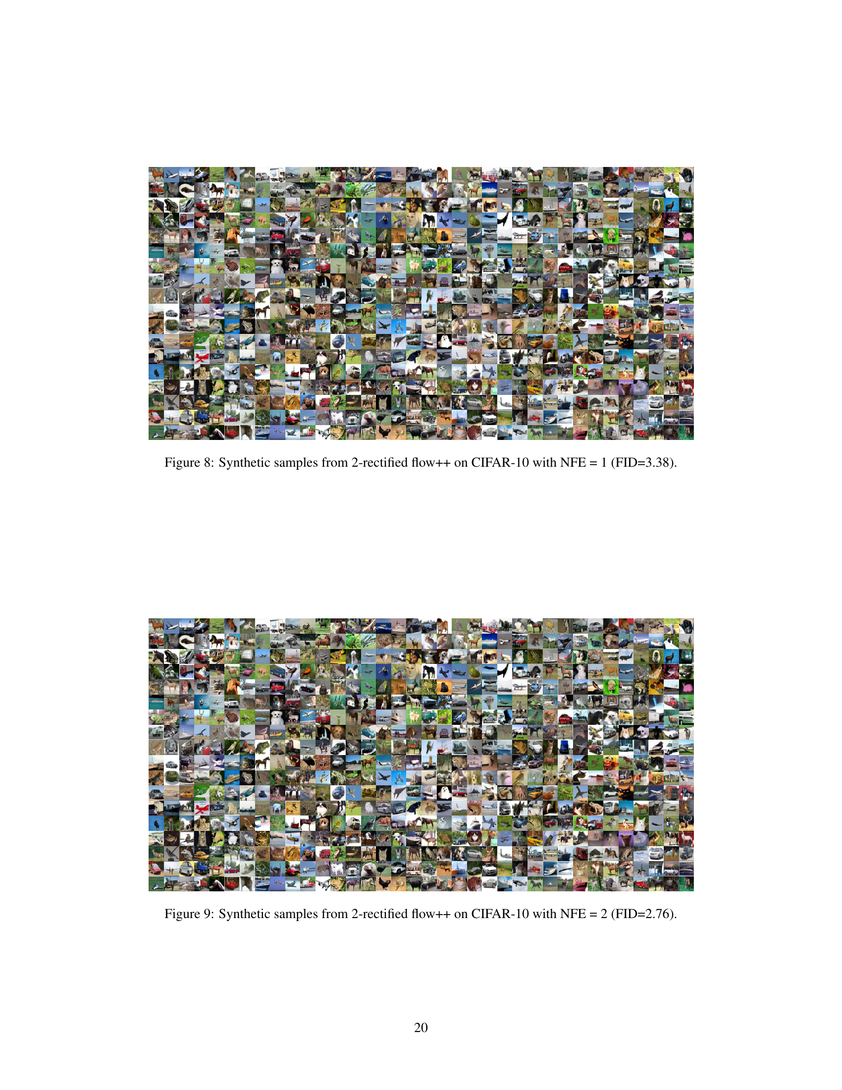
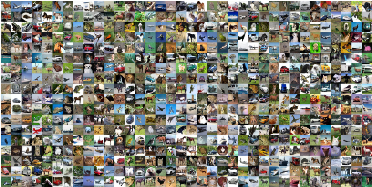
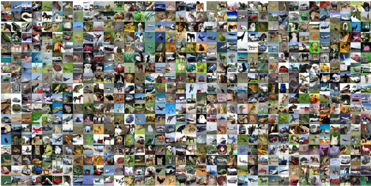
🔼 This figure shows a grid of 2500 synthetic images generated by the 2-rectified flow++ model trained on the CIFAR-10 dataset. The images were generated using only one function evaluation (NFE), and the model achieved a Fréchet Inception Distance (FID) score of 3.38. A lower FID score indicates that the generated images are more realistic and closer in distribution to real CIFAR-10 images.
read the caption
Figure 8: Synthetic samples from 2-rectified flow++ on CIFAR-10 with NFE = 1 (FID=3.38).
🔼 This figure illustrates the rectified flow process. Panel (a) shows linear interpolation between two distributions. Panel (b) shows how rectified flow modifies the trajectories to avoid intersections. Panel (c) shows linear interpolation using samples from the modified distribution, and Panel (d) demonstrates the iterative application of rectified flow (Reflow) to further straighten the trajectories.
read the caption
Figure 1: Rectified flow process (figure modified from Liu et al. [2022]). Rectified flow rewires trajectories so there are no intersecting trajectories (a) → (b). Then, we take noise samples from pz and their generated samples from px, and linearly interpolate them (c). In Reflow, rectified flow is applied again (c) → (d) to straighten flows. This procedure is repeated recursively.
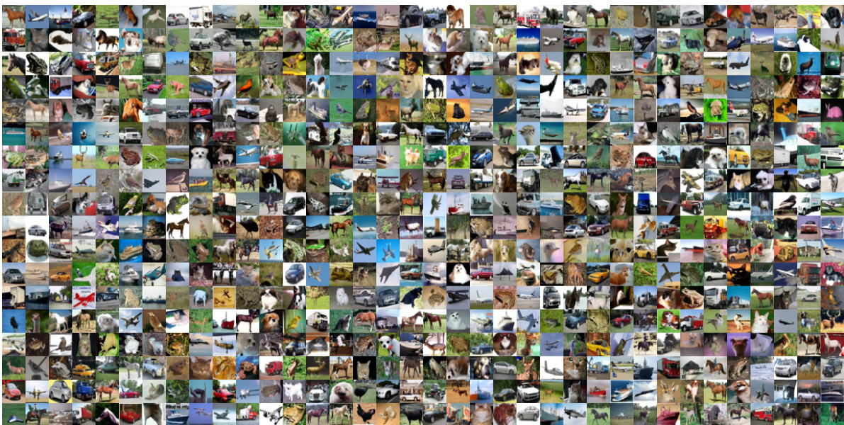
🔼 This figure displays a grid of 100 images generated from the 2-rectified flow++ model trained on the CIFAR-10 dataset. Each image is a synthetic sample produced using only one function evaluation (NFE). The FID (Frechet Inception Distance) score of 3.38 indicates good image quality for such a low computational cost.
read the caption
Figure 8: Synthetic samples from 2-rectified flow++ on CIFAR-10 with NFE = 1 (FID=3.38).
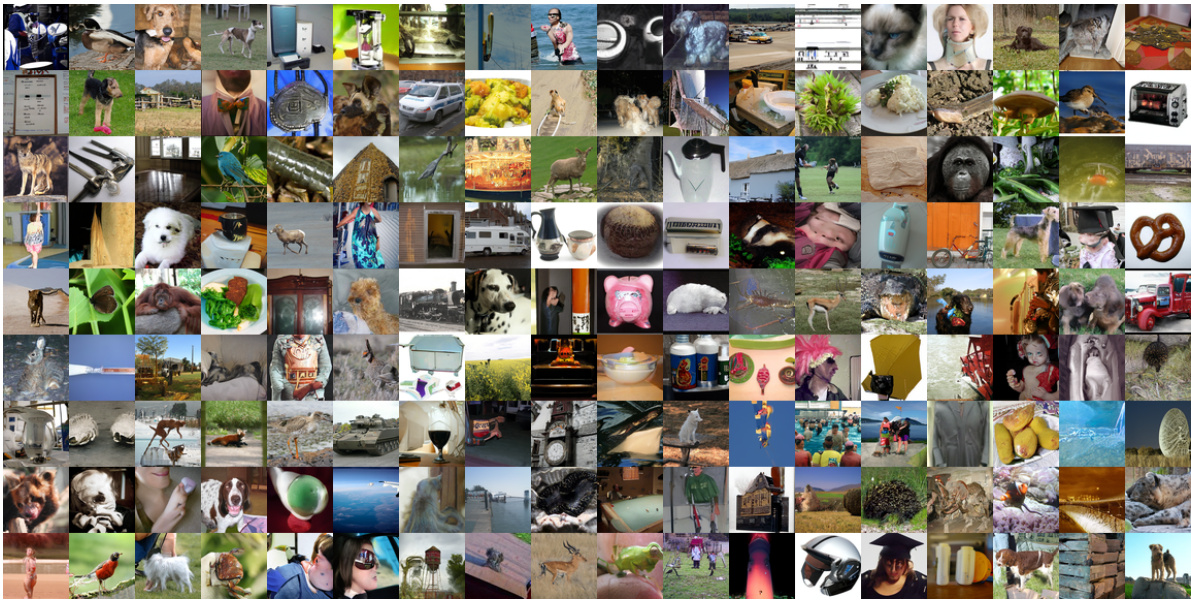
🔼 This figure displays a grid of 256 synthetic images generated using the improved 2-rectified flow++ method. The images are generated from a single forward pass (NFE = 1) and achieve a Fréchet Inception Distance (FID) score of 3.38, demonstrating the model’s ability to generate high-quality images with minimal computational cost.
read the caption
Figure 8: Synthetic samples from 2-rectified flow++ on CIFAR-10 with NFE = 1 (FID=3.38).

🔼 This figure displays a grid of 2500 synthetic images generated using the 2-rectified flow++ method on the CIFAR-10 dataset. The images were generated using only one function evaluation (NFE). The FID (Fréchet Inception Distance) score, a measure of image quality, is 3.38, indicating reasonable image generation quality considering the limited computational resources (1 NFE).
read the caption
Figure 8: Synthetic samples from 2-rectified flow++ on CIFAR-10 with NFE = 1 (FID=3.38).

🔼 This figure displays a grid of 2500 synthetic images generated using the proposed 2-rectified flow++ method on the CIFAR-10 dataset. The images were generated using only a single function evaluation (NFE=1). The FID (Fréchet Inception Distance) score of 3.38 indicates the quality of the generated images relative to the real CIFAR-10 images; lower scores suggest better image quality.
read the caption
Figure 8: Synthetic samples from 2-rectified flow++ on CIFAR-10 with NFE = 1 (FID=3.38).
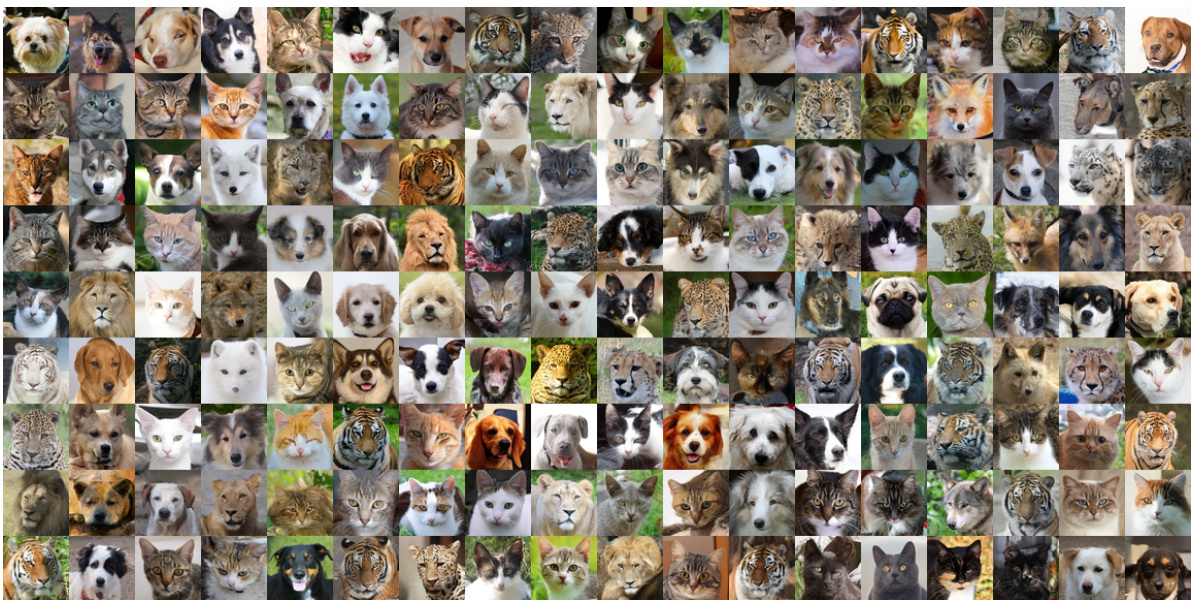
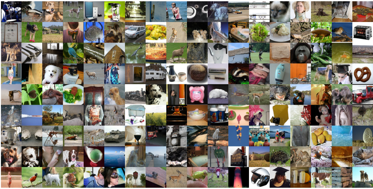
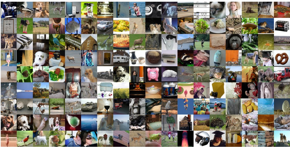
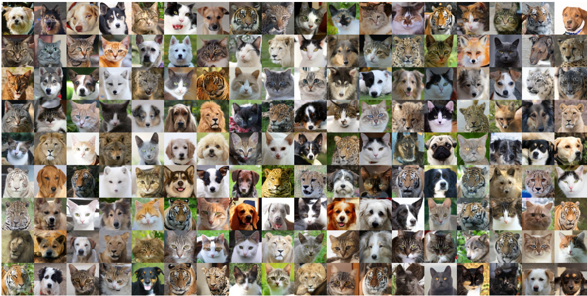
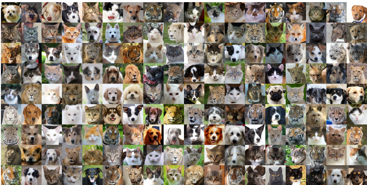
🔼 This figure shows a grid of 256 synthetic images of animals generated by the 2-rectified flow++ model. These images are from the AFHQ 64×64 dataset, and the model was run with only one function evaluation (NFE). The FID score of 4.11 indicates a relatively high quality of image generation compared to other methods at similar NFEs.
read the caption
Figure 16: Synthetic samples from 2-rectified flow++ on AFHQ 64×64 with NFE = 1 (FID=4.11).
🔼 This figure illustrates the rectified flow process, showing how it iteratively refines ODE trajectories to be less susceptible to truncation errors. Panel (a) shows linear interpolation trajectories between two distributions. Panel (b) shows the generative process of a 1-rectified flow that removes trajectory intersections. Panel (c) shows linear interpolation using the generated samples from the 1-rectified flow. Panel (d) shows the generative process of a 2-rectified flow where the process is repeated recursively.
read the caption
Figure 1: Rectified flow process (figure modified from Liu et al. [2022]). Rectified flow rewires trajectories so there are no intersecting trajectories (a) → (b). Then, we take noise samples from pz and their generated samples from px, and linearly interpolate them (c). In Reflow, rectified flow is applied again (c) → (d) to straighten flows. This procedure is repeated recursively.
🔼 This figure illustrates the rectified flow process, showing how it iteratively refines trajectories to make them straighter. Panel (a) shows linear interpolation between two distributions (px and pz), (b) shows the effect of applying rectified flow once to remove intersecting trajectories. (c) illustrates the linear interpolation performed after applying rectified flow. (d) shows the result after recursively applying rectified flow multiple times. The process iteratively straightens the trajectories which makes sampling from the model more efficient.
read the caption
Figure 1: Rectified flow process (figure modified from Liu et al. [2022]). Rectified flow rewires trajectories so there are no intersecting trajectories (a) → (b). Then, we take noise samples from pz and their generated samples from px, and linearly interpolate them (c). In Reflow, rectified flow is applied again (c) → (d) to straighten flows. This procedure is repeated recursively.

🔼 This figure illustrates the rectified flow process, showing how it iteratively learns smooth ODE paths to reduce truncation error. Panel (a) shows linear interpolation between two distributions, (b) shows how rectified flow modifies trajectories to remove intersections, (c) shows linear interpolation of noise samples and their corresponding generated samples, and (d) depicts the iterative refinement process (Reflow) for straightening the flow.
read the caption
Figure 1: Rectified flow process (figure modified from Liu et al. [2022]). Rectified flow rewires trajectories so there are no intersecting trajectories (a) → (b). Then, we take noise samples from pz and their generated samples from px, and linearly interpolate them (c). In Reflow, rectified flow is applied again (c) → (d) to straighten flows. This procedure is repeated recursively.
🔼 This figure shows the inversion results of the proposed method on CIFAR-10 dataset. The reconstruction error is measured using MSE. The distribution of the norm of the inverted noise is shown to evaluate the quality of the inversion process. Finally, the inversion and reconstruction results are shown visually, demonstrating the quality of the inversion. The method outperforms EDM, which fails to produce realistic noise with only 8 NFEs.
read the caption
Figure 5: Inversion results on CIFAR-10. (a) Reconstruction error between real and reconstructed data is measured by the mean squared error (MSE), where the x-axis represents NFEs used for inversion and reconstruction (e.g. 2 means 2 for inversion and 2 for reconstruction). (b) Distribution of ||z||2 of the inverted noises as a proxy for Gaussianity (NFE = 8). The green histogram represents the distribution of true noise, which is Chi-squared with 3 × 32 × 32 = 3072 degrees of freedom. (c) Inversion and reconstruction results using (8 + 8) NFEs. With only 8 NFES, EDM fails to produce realistic noise, and also the reconstructed samples are blurry.
More on tables

🔼 This table presents the results of an ablation study evaluating different training techniques for 2-rectified flows on three datasets: CIFAR-10, AFHQ 64x64, and FFHQ 64x64. It shows how FID (Frechet Inception Distance), a metric for image quality, changes with different training techniques, including different loss functions and timestep distributions, both for one and two NFE (number of function evaluations). The baseline uses the squared l2 distance and a uniform timestep distribution. The improved configurations show the FID improvements sequentially as each technique is applied.
read the caption
Table 1: Effects of the improved training techniques. The baseline (config A) is the 2-rectified flow with the uniform timestep distribution and the squared l2 metric [Liu et al., 2022]. Config B is the improved baseline with EDM initialization (Sec. 4.3) and increased batch size (128 → 512 on CIFAR-10). FID (the lower the better) is computed using 50,000 synthetic samples and the entire training set. We train the models for 800,000 iterations on CIFAR-10 and 1,000,000 iterations on AFHQ and FFHQ and report the best FID for each setting.
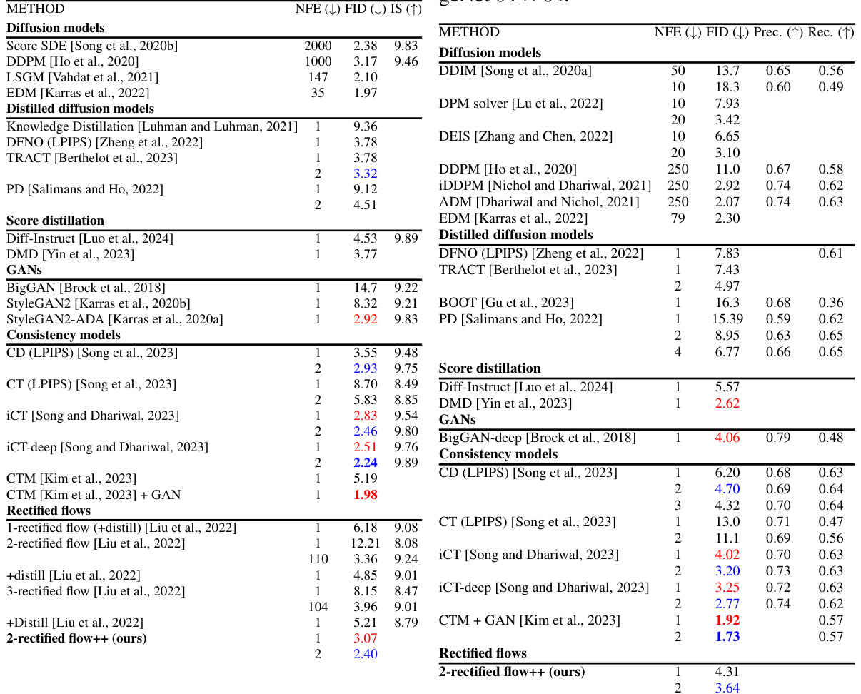
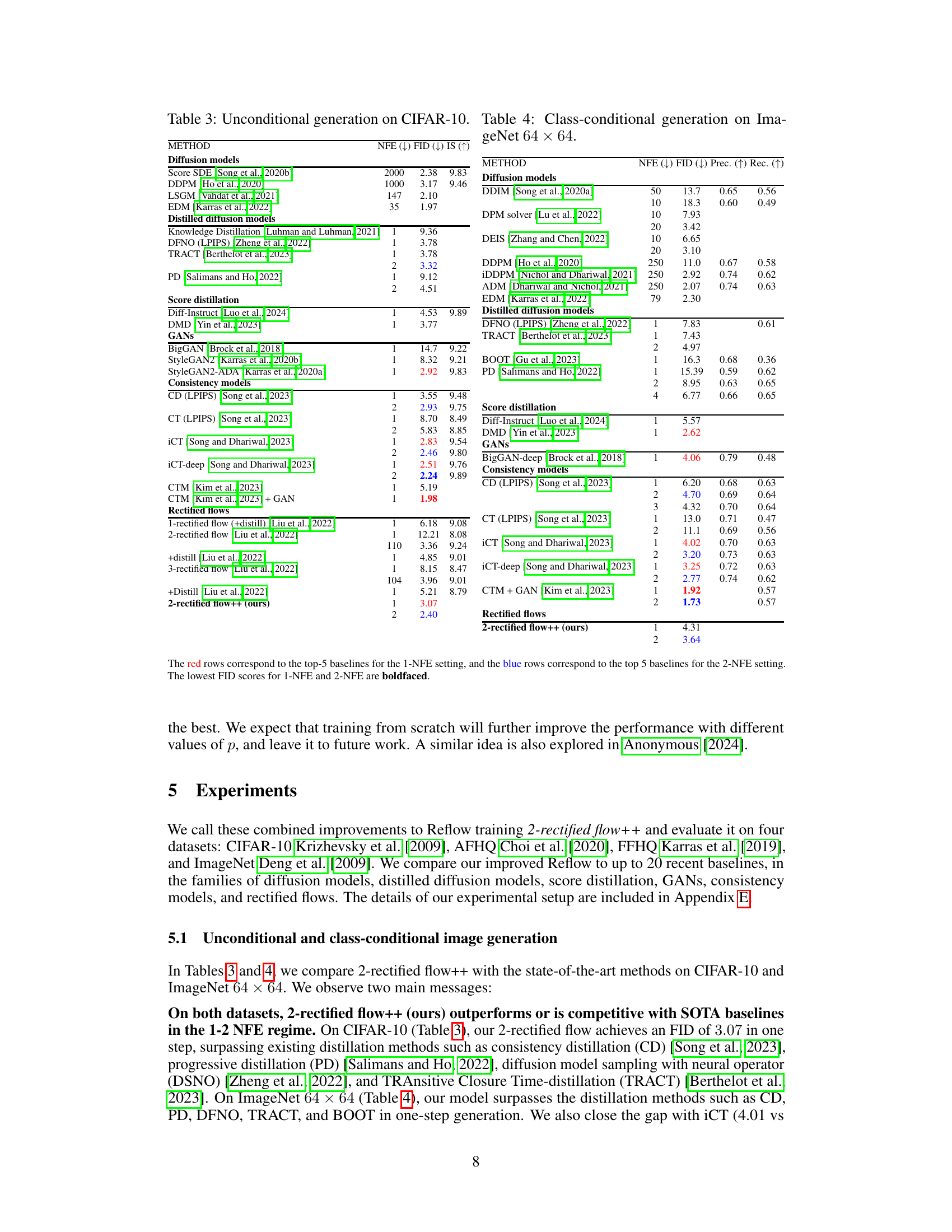
🔼 This table presents a comparison of unconditional image generation results on CIFAR-10 and class-conditional image generation results on ImageNet 64x64. It compares various methods, including diffusion models, distilled diffusion models, GANs, consistency models, and rectified flows, across different numbers of function evaluations (NFEs), evaluating performance using FID (Frechet Inception Distance) and, where applicable, Inception Score (IS), Precision, and Recall.
read the caption
Table 3: Unconditional generation on CIFAR-10. Table 4: Class-conditional generation on ImageNet 64 × 64.

🔼 This table compares the computational cost of Reflow with two other distillation methods, CD and CT, in terms of the number of forward passes required during training. It shows that while Reflow initially requires generating synthetic data-noise pairs, the overall number of forward passes for Reflow is lower than CD and slightly lower than CT, suggesting Reflow could be computationally efficient despite this initial step.
read the caption
Table 6: Comparison of the number of forward passes. Reflow uses 395M forward passes for generating pairs and 1, 433.6M for training.

🔼 This table presents the effects of various training techniques on the performance of 2-rectified flow. It compares a baseline configuration with several improved variations, showing the impact of different timestep distributions, loss functions, and initializations. The results are measured by FID scores across three datasets: CIFAR-10, AFHQ 64x64, and FFHQ 64x64.
read the caption
Table 1: Effects of the improved training techniques. The baseline (config A) is the 2-rectified flow with the uniform timestep distribution and the squared l2 metric [Liu et al., 2022]. Config B is the improved baseline with EDM initialization (Sec. 4.3) and increased batch size (128 → 512 on CIFAR-10). FID (the lower the better) is computed using 50,000 synthetic samples and the entire training set. We train the models for 800,000 iterations on CIFAR-10 and 1,000,000 iterations on AFHQ and FFHQ and report the best FID for each setting.
Full paper#
