TL;DR#
Many methods using machine learning to solve scientific problems based on partial differential equations (PDEs) are data intensive and computationally expensive. This requires a large amount of PDE data, which needs expensive numerical PDE solutions. This partially undermines the original goal of avoiding these expensive simulations. This paper addresses this data efficiency challenge in scientific machine learning by proposing unsupervised pretraining for PDE operator learning to reduce the need for training data.
To improve the data efficiency, the authors propose unsupervised pretraining for neural operator learning on unlabeled PDE data without simulated solutions to reduce the need for training data with heavy simulation costs. Physics-inspired reconstruction-based proxy tasks are used to pretrain neural operators. In addition, they propose a similarity-based method for in-context learning that allows neural operators to flexibly leverage in-context examples without incurring extra training costs or designs. Extensive empirical evaluations on various PDEs demonstrate that their method is highly data-efficient, generalizable, and outperforms conventional vision-pretrained models.
Key Takeaways#
Why does it matter?#
This paper is crucial because it tackles the data inefficiency problem in scientific machine learning, a significant hurdle in applying machine learning to complex scientific problems. By introducing unsupervised pretraining and in-context learning, it offers a highly effective and data-efficient approach to solving partial differential equations, significantly reducing simulation costs while improving accuracy and generalization. This opens exciting new avenues for research by making advanced PDE solutions more accessible and cost-effective.
Visual Insights#

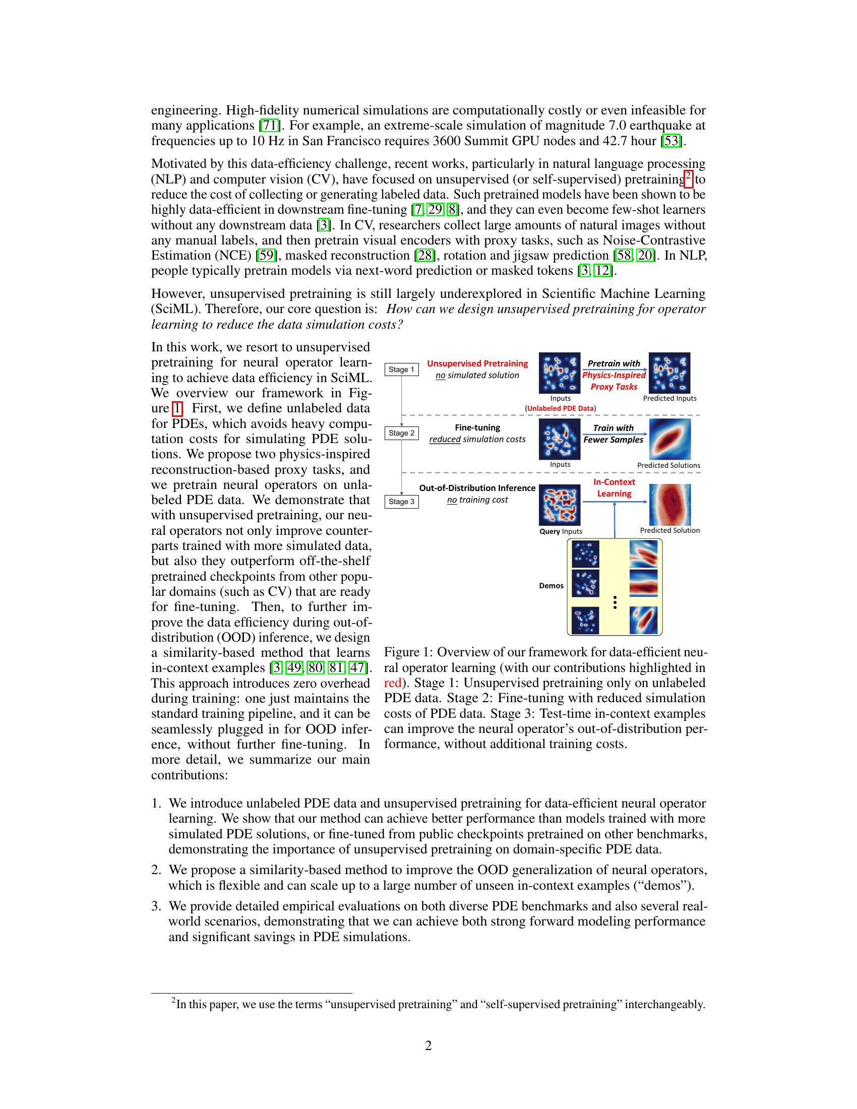
🔼 This figure illustrates the three stages of the proposed data-efficient neural operator learning framework. Stage 1 involves unsupervised pretraining on unlabeled PDE data using physics-inspired proxy tasks. Stage 2 performs fine-tuning with reduced simulation costs on labeled PDE data. Finally, stage 3 leverages in-context learning during inference to improve out-of-distribution performance without additional training. The contributions of the authors are highlighted in red.
read the caption
Figure 1: Overview of our framework for data-efficient neural operator learning (with our contributions highlighted in red). Stage 1: Unsupervised pretraining only on unlabeled PDE data. Stage 2: Fine-tuning with reduced simulation costs of PDE data. Stage 3: Test-time in-context examples can improve the neural operator’s out-of-distribution performance, without additional training costs.

🔼 This table summarizes the input and output data used for training neural operators on various partial differential equations (PDEs). It shows the input features (e.g., source function, diffusion coefficients, vorticity, spatiotemporal coordinates) and the corresponding output targets (e.g., potential field, wave function, velocity, pressure) for each PDE. The table also provides abbreviations for the PDE names: NS for Navier-Stokes and RD for Reaction-Diffusion. Table 3, referenced in this caption, provides the resolution details of the data.
read the caption
Table 1: Inputs and outputs for learning different PDEs. See Table 3 for resolutions. 'NS': Navier-Stokes. “RD': Reaction-Diffusion.
In-depth insights#
Unsupervised PDE#
The concept of “Unsupervised PDE” learning is intriguing and potentially transformative. It addresses the core challenge of data scarcity in scientific machine learning, especially within the context of partial differential equations (PDEs). Traditional PDE-solving methods using supervised learning require massive, computationally expensive datasets of simulated solutions. Unsupervised approaches, however, aim to leverage unlabeled data, such as physical parameters or initial conditions without corresponding solutions, to learn useful representations. This significantly reduces the computational burden and opens possibilities for applications where generating labeled data is infeasible. The key lies in developing effective proxy tasks which allow a neural network to learn the underlying structure of the PDE system without needing explicit solutions. This requires domain-specific knowledge to design such tasks that capture the essence of PDE dynamics, making the approach both data efficient and potentially more generalizable to unseen or out-of-distribution scenarios. Success in unsupervised PDE learning could lead to significant breakthroughs in areas such as weather forecasting, fluid dynamics, and material science.
Proxy Task Design#
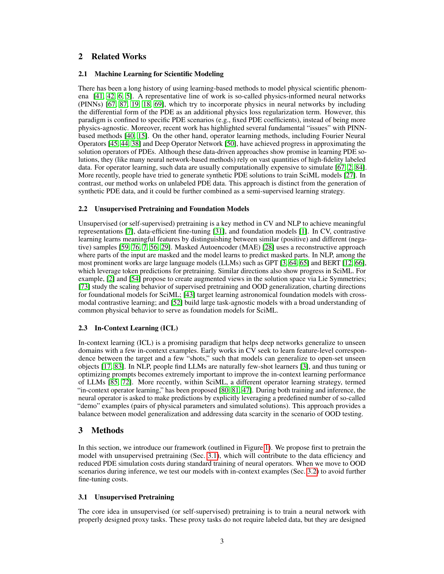
The effectiveness of unsupervised pretraining hinges on the ingenuity of the proxy tasks. The paper cleverly employs two physics-inspired reconstruction-based tasks: Masked Autoencoders (MAE) and Super-Resolution (SR). MAE leverages the inherent invariance of PDEs to sparse sensing by randomly masking portions of the input data and training the network to reconstruct the complete signal. This approach forces the model to learn robust, spatially invariant representations. SR addresses the challenge of resolution invariance, a common feature in real-world scientific datasets. By introducing blurring to the input, SR encourages the network to learn features robust to variations in resolution, thereby improving generalization. The choice of these tasks is not arbitrary; they directly reflect the characteristics of PDE data and are designed to promote data efficiency and generalization to unseen examples during downstream supervised training.
In-context Learning#
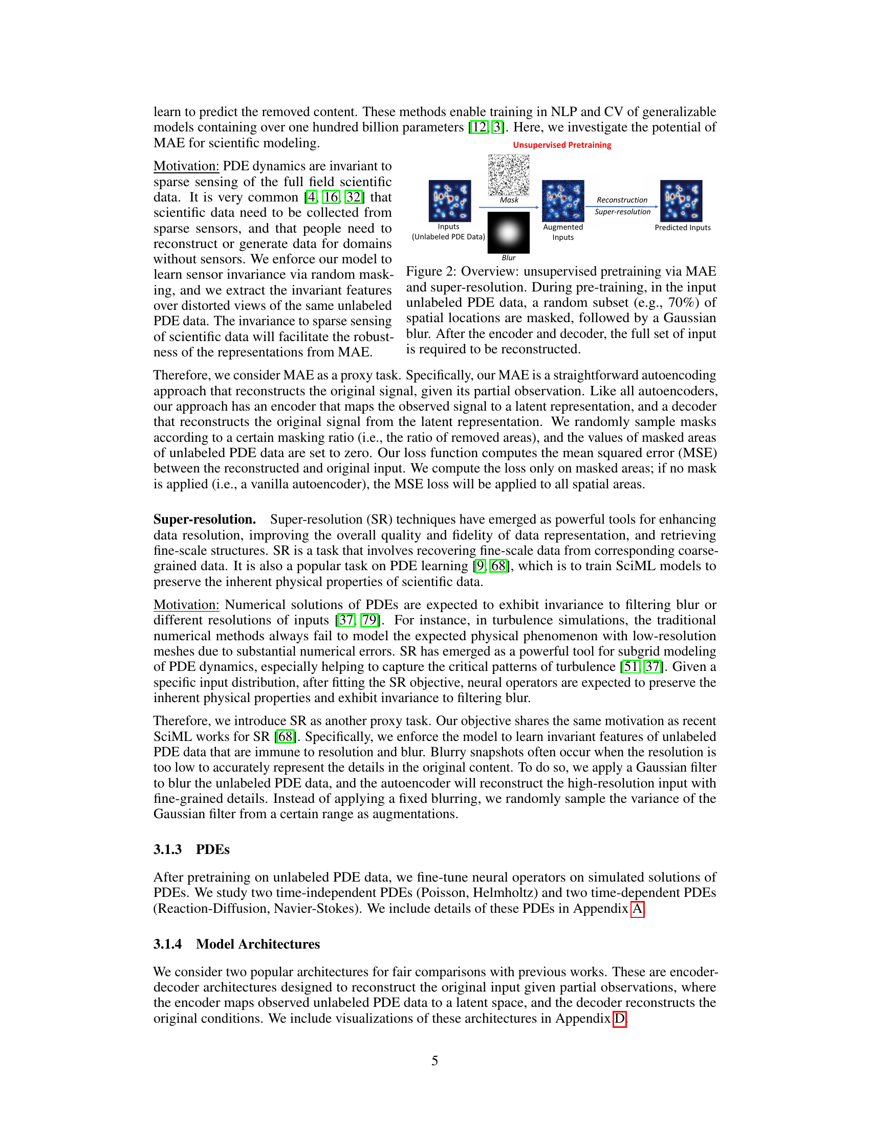
In-context learning (ICL) offers a compelling paradigm shift in machine learning, particularly for tackling challenges in data-scarce domains like scientific machine learning (SciML). Instead of relying solely on extensive pre-training and fine-tuning, ICL leverages a few in-context examples (‘demos’) provided alongside the query input at inference time. This approach dramatically reduces the need for extensive labeled training data, enhancing efficiency and lowering simulation costs in computationally expensive areas like solving PDEs. The mechanism by which ICL improves out-of-distribution (OOD) generalization is multifaceted; it appears to involve flexible adaptation based on similarity between query and demos, enabling operators to flexibly incorporate novel data without retraining. Although similarity-based methods appear effective, ICL methods lack theoretical guarantees, making it crucial to carefully explore this methodology’s strengths and limitations. Further research should focus on developing a stronger theoretical underpinning and exploring different similarity metrics for optimal performance. Despite these unknowns, ICL represents a promising avenue for increasing the practicality and effectiveness of operator learning for complex scientific problems.
Real-world Testing#
A dedicated ‘Real-world Testing’ section would significantly enhance the paper’s impact. It should present evaluations on datasets representing realistic, complex scenarios beyond the controlled benchmarks. Diverse data types are crucial: this includes incorporating noisy data, incomplete datasets, and varying resolutions – situations frequently encountered in practice. The evaluation should go beyond simple metrics, delving into the robustness and generalizability of the proposed methods under these conditions. Analyzing failure modes in such realistic environments is vital. Does the method exhibit graceful degradation or catastrophic failures? How do these failures relate to specific characteristics of the real-world data? Comparisons against existing methods, not only in terms of accuracy but also in robustness to data variations, should be included. Finally, a discussion on the practical implications of the findings is key. How does the performance on real-world data translate into tangible benefits or limitations for users in the respective fields?
Future of SciML#
The future of Scientific Machine Learning (SciML) is bright, but also faces significant challenges. Data efficiency will remain a key focus, with further research into unsupervised and self-supervised learning techniques crucial for reducing reliance on expensive simulations. Improved generalizability is another priority; current methods often struggle with out-of-distribution inference. Incorporating physics-informed priors more effectively will improve model accuracy and reduce the need for massive datasets. Developing more robust and scalable methods for handling high-dimensional and complex systems is essential. Explainability and interpretability must improve for wider acceptance, particularly in scientific contexts demanding trust and validation. The integration of SciML with other domains, such as high-performance computing, will be crucial for scaling up to real-world applications. Finally, interdisciplinary collaboration between machine learning researchers and domain experts will be vital for driving meaningful progress in SciML’s diverse and challenging landscape.
More visual insights#
More on figures
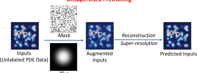
🔼 This figure illustrates the unsupervised pretraining framework using Masked Autoencoders (MAE) and super-resolution. The process begins with input unlabeled PDE data. A portion of the data is randomly masked (e.g., 70%), and a Gaussian blur is applied to the masked regions. This modified data is then passed through an encoder and decoder network. The decoder’s task is to reconstruct the original input data from the masked and blurred version, forcing the model to learn robust and invariant features despite data corruption. This method helps the model become more resilient to sparse or noisy data, common in scientific applications.
read the caption
Figure 2: Overview: unsupervised pretraining via MAE and super-resolution. During pre-training, in the input unlabeled PDE data, a random subset (e.g., 70%) of spatial locations are masked, followed by a Gaussian blur. After the encoder and decoder, the full set of input is required to be reconstructed.
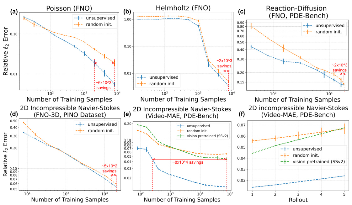
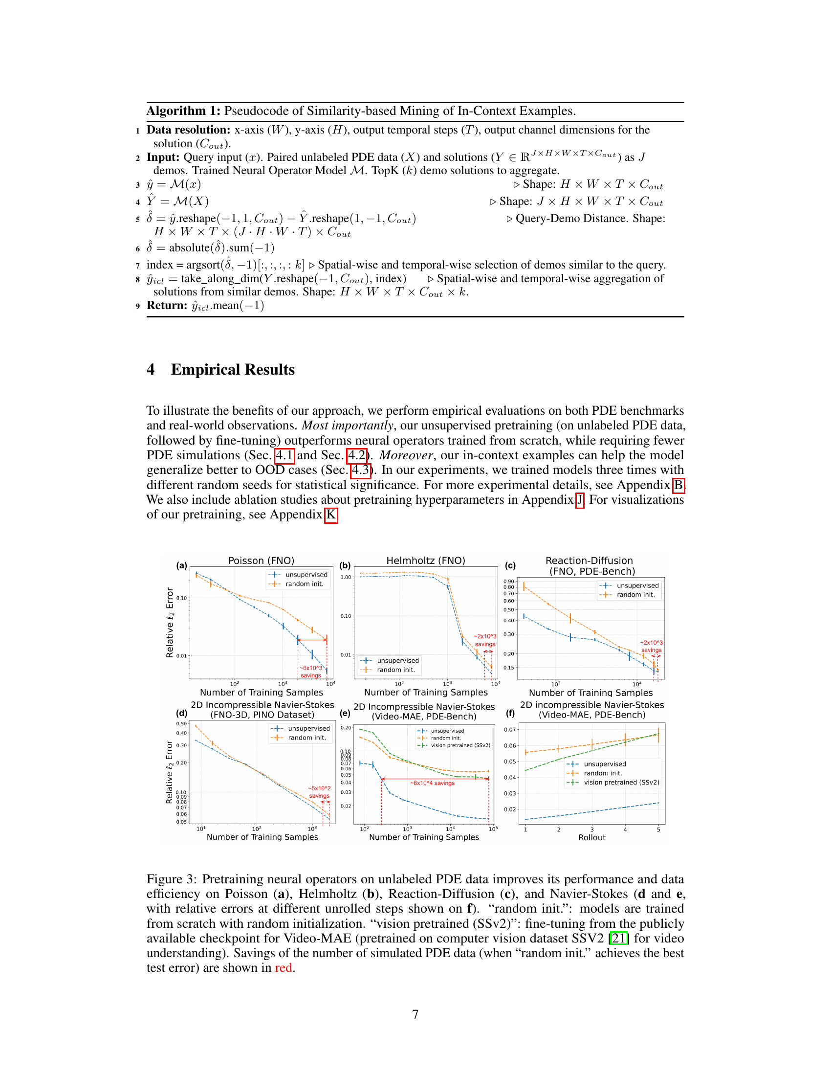
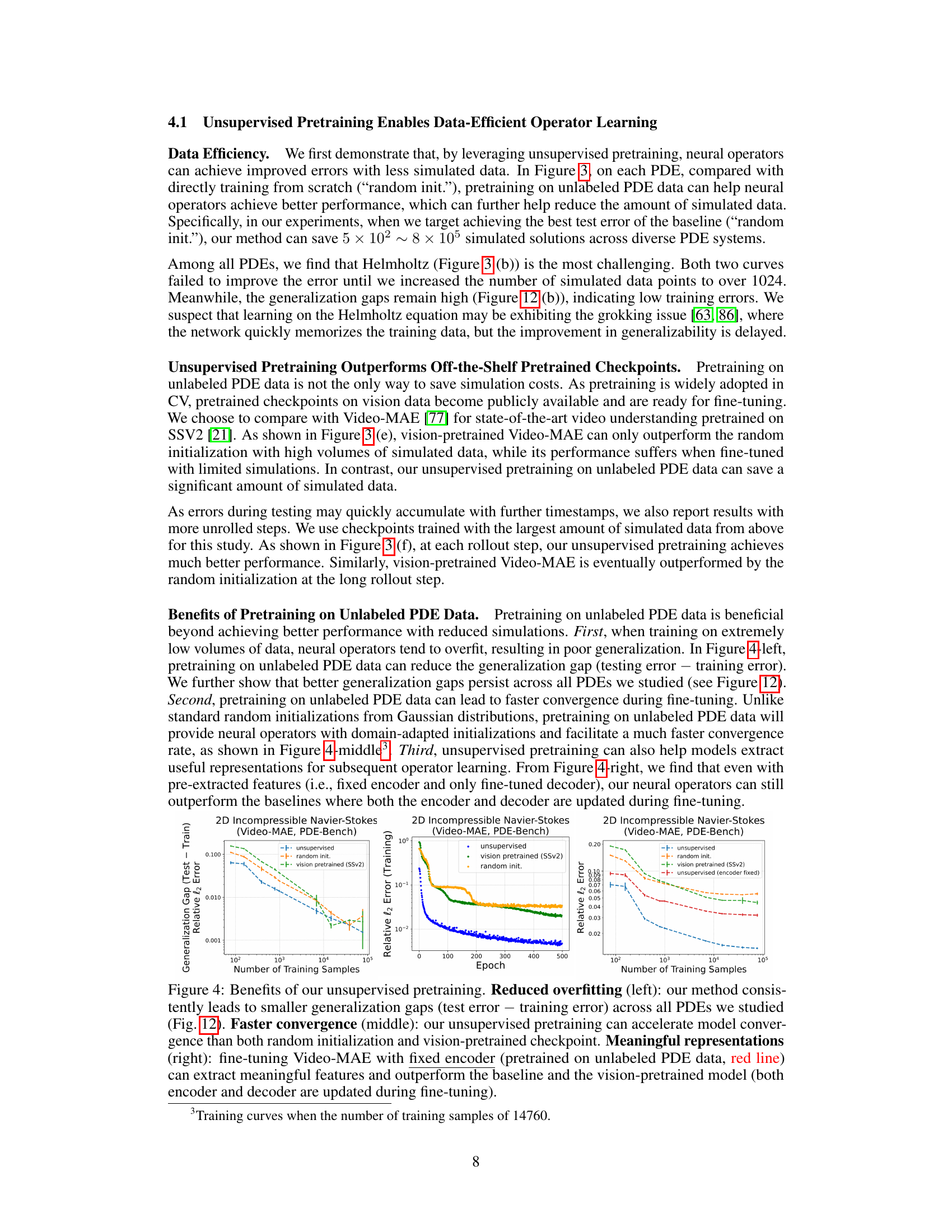
🔼 This figure demonstrates the data efficiency of unsupervised pretraining for neural operators on various PDEs. It compares the performance of models trained from scratch (‘random init.’) against models with unsupervised pretraining and those fine-tuned from a vision-pretrained model (SSv2). The results show that unsupervised pretraining significantly reduces the number of simulated PDE data needed to achieve comparable or better performance than models trained from scratch, highlighting its data efficiency. The savings in the number of simulated data points are shown in red.
read the caption
Figure 3: Pretraining neural operators on unlabeled PDE data improves its performance and data efficiency on Poisson (a), Helmholtz (b), Reaction-Diffusion (c), and Navier-Stokes (d and e, with relative errors at different unrolled steps shown on f). 'random init.': models are trained from scratch with random initialization. “vision pretrained (SSv2)': fine-tuning from the publicly available checkpoint for Video-MAE (pretrained on computer vision dataset SSV2 [21] for video understanding). Savings of the number of simulated PDE data (when 'random init.' achieves the best test error) are shown in red.

🔼 This figure compares the performance of three different neural operator training methods across various PDEs: unsupervised pretraining, training from scratch (‘random init.’), and fine-tuning a vision-pretrained model. The results show that unsupervised pretraining using unlabeled data significantly improves performance and reduces the need for simulated data, leading to greater data efficiency. The figure also highlights that, for the same level of performance, the number of training samples required is substantially less when using unsupervised pretraining, resulting in significant savings of simulation costs.
read the caption
Figure 3: Pretraining neural operators on unlabeled PDE data improves its performance and data efficiency on Poisson (a), Helmholtz (b), Reaction-Diffusion (c), and Navier-Stokes (d and e, with relative errors at different unrolled steps shown on f). 'random init.': models are trained from scratch with random initialization. “vision pretrained (SSv2)': fine-tuning from the publicly available checkpoint for Video-MAE (pretrained on computer vision dataset SSV2 [21] for video understanding). Savings of the number of simulated PDE data (when 'random init.' achieves the best test error) are shown in red.

🔼 This figure demonstrates the data efficiency gains achieved by unsupervised pretraining of neural operators on unlabeled PDE data. It compares the performance of models trained from scratch (‘random init.’) and those fine-tuned from a vision-pretrained model (SSv2) against models using the unsupervised pretraining method. The plots show relative l2 error versus the number of training samples for various PDEs (Poisson, Helmholtz, Reaction-Diffusion, Navier-Stokes). The red numbers highlight the significant reduction in the number of simulated PDE data required to achieve comparable or better performance with the unsupervised pretraining method.
read the caption
Figure 3: Pretraining neural operators on unlabeled PDE data improves its performance and data efficiency on Poisson (a), Helmholtz (b), Reaction-Diffusion (c), and Navier-Stokes (d and e, with relative errors at different unrolled steps shown on f). 'random init.': models are trained from scratch with random initialization. “vision pretrained (SSv2)': fine-tuning from the publicly available checkpoint for Video-MAE (pretrained on computer vision dataset SSV2 [21] for video understanding). Savings of the number of simulated PDE data (when 'random init.' achieves the best test error) are shown in red.

🔼 This figure shows the architectures of two neural operator models used in the paper: the Fourier Neural Operator (FNO) and the Video-MAE. The FNO architecture uses a series of Fourier layers, while the Video-MAE uses a transformer-based encoder-decoder structure. Both are designed for processing spatiotemporal data. The detailed components of each architecture, including linear layers, activation functions (GeLU), and Fourier transforms, are illustrated. This visualization helps clarify the structural differences between these two prominent deep learning models used in the experiments.
read the caption
Figure 7: Visualizations of architectures we studied. Left: FNO [46]. Right: VideoMAE [77].

🔼 This figure compares the performance of the proposed unsupervised pretraining method against MoCo v2, a popular contrastive learning method, on the ERA5 dataset. The x-axis represents the number of training samples used, and the y-axis shows the relative l2 error. The plot demonstrates that the unsupervised pretraining method consistently achieves lower error rates than MoCo v2 across varying training data sizes, highlighting its superior data efficiency.
read the caption
Figure 8: Comparison between our unsupervised pretraining method versus MoCo v2 [8].

🔼 This figure compares the performance of three different training methods for neural operators on Poisson and Helmholtz PDEs. The ‘random init.’ method trains the model from scratch with random weights, showing a clear need for substantial training data to achieve good performance. The ‘vision pretrained’ method uses a model pre-trained on ImageNet, a large computer vision dataset, before fine-tuning it on the PDE data. This approach shows some improvement over the random initialization, but is still not as efficient as the ‘unsupervised’ method. The ‘unsupervised’ method uses a model pre-trained on unlabeled PDE data before fine-tuning, showing significant performance gains with far less training data than the other methods. This demonstrates the effectiveness of unsupervised pre-training on the specific domain of PDEs.
read the caption
Figure 9: Pretraining neural operators on unlabeled PDE data improves its performance and data efficiency on Poisson (left), Helmholtz (right). 'random init.': models are trained from scratch with random initialization. 'vision pretrained': fine-tuning from the checkpoint pretrained on computer vision dataset ImageNet [11].

🔼 This figure shows the results of an experiment comparing the performance of neural operators trained with different pretraining strategies. The green line represents a model pretrained on a combination of unlabeled Poisson, Helmholtz, and Navier-Stokes datasets (joint pretraining), while the other lines show results for models pretrained on single unlabeled datasets or trained from scratch (‘random init.’). The results demonstrate that joint pretraining leads to superior performance and data efficiency during fine-tuning on various PDEs (Poisson, Helmholtz, and Reaction-Diffusion).
read the caption
Figure 10: Joint unsupervised pretraining on multiple PDEs (green solid curve) further improves the data efficiency of neural operators when fine-tuning on Poisson (left), Helmholtz (middle), Reaction-Diffusion (right). 'random init.': models are trained from scratch with random initialization. 'unsupervised': models are pretrained on a single unsupervised PDE data. 'unsupervised joint': models are pretrained on a joint of multiple unsupervised PDE datasets. 'NS': Navier Stokes. 'RD': Reaction-Diffusion.
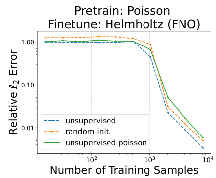
🔼 This figure shows the results of fine-tuning a Fourier Neural Operator (FNO) model, pretrained on the Poisson equation, on the Helmholtz equation. It compares the performance of the model with unsupervised pretraining on the Poisson data to a model trained from scratch (‘random init.’) and a model fine-tuned from an ImageNet-pretrained checkpoint. The x-axis represents the number of training samples, and the y-axis represents the relative l2 error. The graph demonstrates that unsupervised pretraining on a related task improves the model’s performance on a new, unseen task, requiring fewer training samples than the other models.
read the caption
Figure 11: Fine-tuning FNO (pretrained on Poisson) on unseen samples from Helmholtz.

🔼 This figure demonstrates the data efficiency and improved performance achieved by pretraining neural operators on unlabeled PDE data. It compares the performance of models trained from scratch (‘random init.’), models fine-tuned from a vision-pretrained model (SSv2), and models using the proposed unsupervised pretraining method. The results are shown across four different PDEs, highlighting significant data savings with the unsupervised pretraining approach.
read the caption
Figure 3: Pretraining neural operators on unlabeled PDE data improves its performance and data efficiency on Poisson (a), Helmholtz (b), Reaction-Diffusion (c), and Navier-Stokes (d and e, with relative errors at different unrolled steps shown on f). 'random init.': models are trained from scratch with random initialization. “vision pretrained (SSv2)': fine-tuning from the publicly available checkpoint for Video-MAE (pretrained on computer vision dataset SSV2 [21] for video understanding). Savings of the number of simulated PDE data (when 'random init.' achieves the best test error) are shown in red.
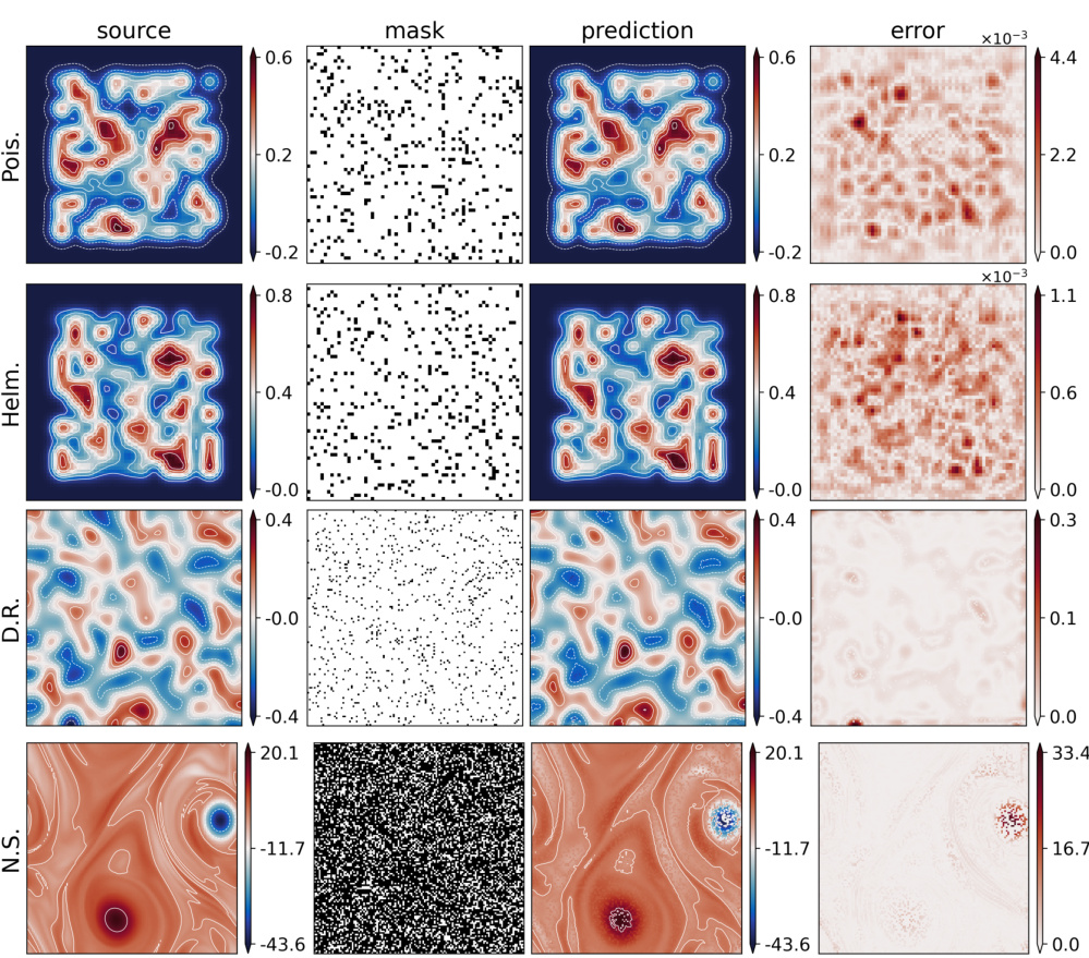
🔼 This figure visualizes the reconstruction performance of the masked autoencoder (MAE) pretraining method on four different types of partial differential equations (PDEs): Poisson, Helmholtz, Reaction-Diffusion, and Navier-Stokes. Each row represents a different PDE. The columns show the original ‘source’ data, the ‘mask’ applied to the data during training (white areas are visible, black areas are masked), the MAE’s ‘prediction’ of the complete data, and the ’error’ between the prediction and the original data. The mask ratio, which indicates the proportion of masked data, varies across the PDEs, reflecting different optimal masking strategies depending on data characteristics.
read the caption
Figure 13: Visualization of FNO reconstructions of unlabeled PDE data on the Poisson ('Pois.'), Helmholtz ('Helm.'), 2D Diffusion-Reaction ('D.R.'), and 2D incompressible Navier-Stokes ('N.S.') equations during MAE pretraining. (Mask ratio: 0.1 for Poisson, Helmholtz, and 2D Diffusion-Reaction equations; 0.7 for incompressible Navier-Stokes.) In masks, only white areas are visible to the model during pretraining.
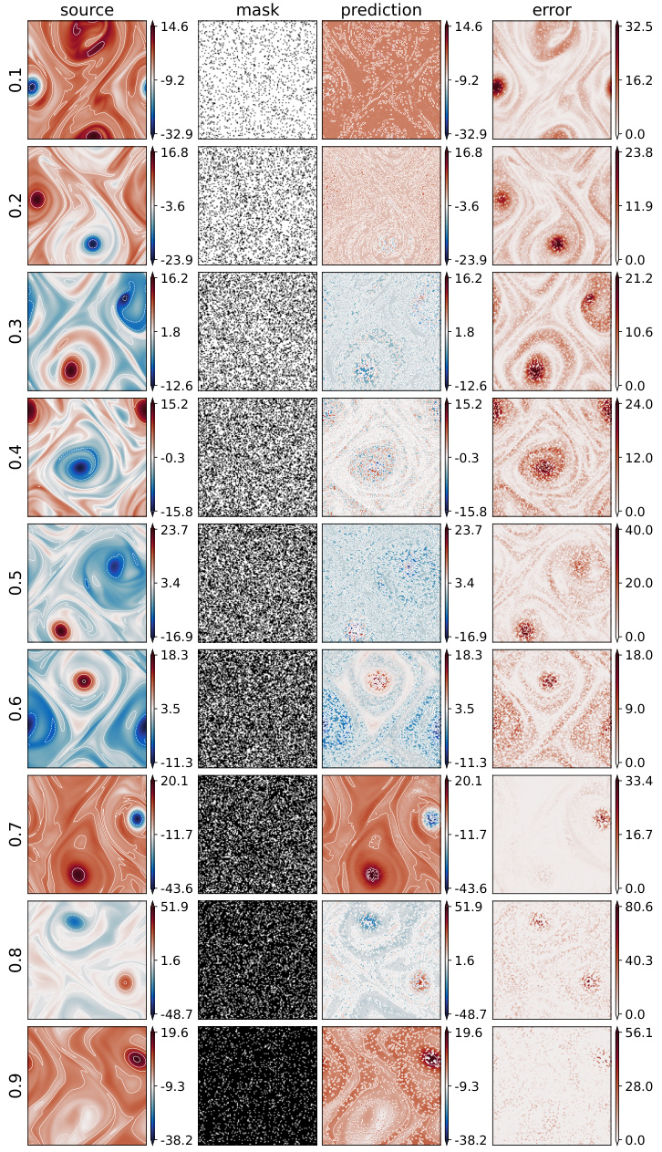
🔼 This figure visualizes the results of masked autoencoder (MAE) pretraining on four different partial differential equations (PDEs). The leftmost column shows the original data (‘source’), the middle column shows the masked data used for training (‘mask’), the third column displays the FNO’s reconstruction of the original data from the masked data (‘prediction’), and the rightmost column shows the difference between the original and reconstructed data (’error’). The masking ratio, which is the percentage of the data masked for training, was varied between PDEs; a more aggressive masking ratio was used for the 2D incompressible Navier-Stokes equation.
read the caption
Figure 13: Visualization of FNO reconstructions of unlabeled PDE data on the Poisson ('Pois.'), Helmholtz ('Helm.'), 2D Diffusion-Reaction ('D.R.'), and 2D incompressible Navier-Stokes ('N.S.') equations during MAE pretraining. (Mask ratio: 0.1 for Poisson, Helmholtz, and 2D Diffusion-Reaction equations; 0.7 for incompressible Navier-Stokes.) In masks, only white areas are visible to the model during pretraining.
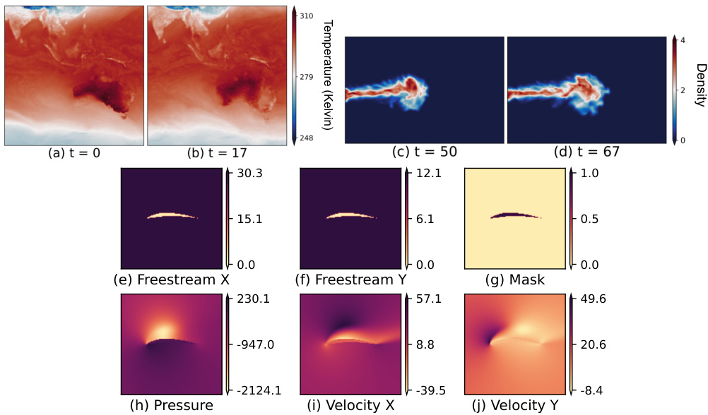
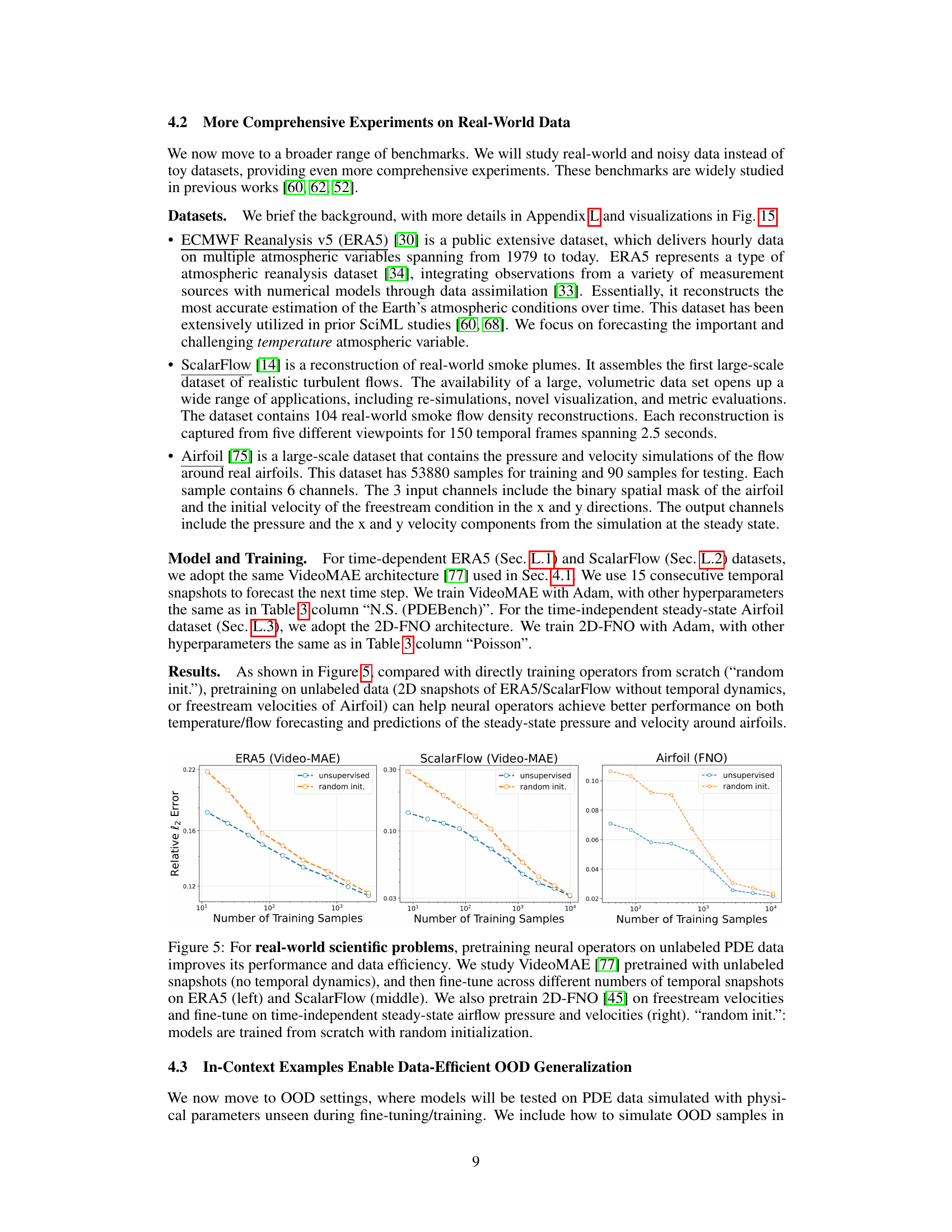
🔼 This figure shows examples of real-world datasets used in the paper. (a, b) show ERA5 temperature data at different timesteps. (c, d) show ScalarFlow density data at different timesteps. (e-j) show the Airfoil dataset, which includes mask, freestream velocity (x and y directions), pressure, and velocity (x and y directions). These examples showcase the variety of data used in the paper’s experiments, representing different physical processes and levels of complexity.
read the caption
Figure 15: We show snapshot examples from ERA5 temperature [30] (a, b) and ScalarFlow [14] (c, d) at different temporal steps; and also an example of Airfoil mask, velocities, and pressure [75] (e-j).

🔼 The figure shows the benefits of using in-context examples in improving the accuracy of PDE prediction. The relative MSE error is decomposed into ‘Scale’ (alignment of model output range with targets) and ‘Shape’ (alignment of scale-invariant structures). The results indicate that adding more demos improves the calibration of model output scale, leading to better accuracy.
read the caption
Figure 16: Benefits of in-context examples. To analyze the benefit of in-context examples for complicated PDE systems, we decompose the relative MSE error into \'Scale\' and \'Shape\'. \'Scale\' indicates the alignment of the range of model outputs with targets (closer to 1 the better), via the slope of a linear regression. \'Shape\' indicates the alignment of scale-invariant spatial/temporal structures via normalized relative MSE (i.e. model outputs or targets are normalized by their own largest magnitude before MSE). We find that the benefit of in-context examples lies in that the scale of the model\'s output keeps being calibrated (red line being closer to 1) when adding more demos.

🔼 This figure visualizes the impact of using in-context examples on the out-of-distribution (OOD) generalization performance of Fourier Neural Operators (FNOs). It shows that incorporating in-context examples improves the accuracy of predictions, particularly in terms of aligning the range of predicted solutions with the true solutions. The differences in solution patterns and value ranges between in-distribution and out-of-distribution data highlight the challenges of OOD generalization for neural operators, and the effectiveness of the proposed in-context learning method.
read the caption
Figure 17: Visualizations of mining in-context examples for FNO in OOD testing. Ranges of solutions predicted with in-context examples (min/max of each snapshot, reflected in colorbars) become closer to the target.
More on tables

🔼 This table provides a summary of the input and output data used for training neural operators on various partial differential equations (PDEs). It shows the different types of PDEs considered (Poisson, Helmholtz, Navier-Stokes, and Reaction-Diffusion), the input features used for each PDE (e.g., source function, diffusion coefficients, vorticity, velocity, pressure), the shape of the input data, and the corresponding target outputs that the model aims to predict. Note that the table refers to Table 3 for the spatial resolution (H x W) of the data which is not provided in this table itself.
read the caption
Table 1: Inputs and outputs for learning different PDEs. See Table 3 for resolutions. 'NS': Navier-Stokes. “RD”: Reaction-Diffusion.

🔼 This table shows the ranges of physical parameters used for different stages of the experiment. The parameters include the diffusion coefficient for Poisson’s equation, the wavenumber for the Helmholtz equation, and the Reynolds number for the Navier-Stokes equation. The ranges are different for unsupervised pretraining, fine-tuning/training, and out-of-distribution testing, reflecting the strategy used to progressively refine the model’s ability to handle different levels of data availability and complexity.
read the caption
Table 2: Ranges of physical parameters (integers) for unsupervised pretraining, training (fine-tuning), and out-of-distribution (OOD) inference.

🔼 This table shows the hyperparameters used for both pretraining and training/fine-tuning stages for various PDEs. It specifies the number of samples, learning rate, batch size, resolution, epochs/iterations, and rollouts used for each PDE and stage. Note the use of D-adaptation for the learning rate in some cases and the dynamic batch size based on the number of samples.
read the caption
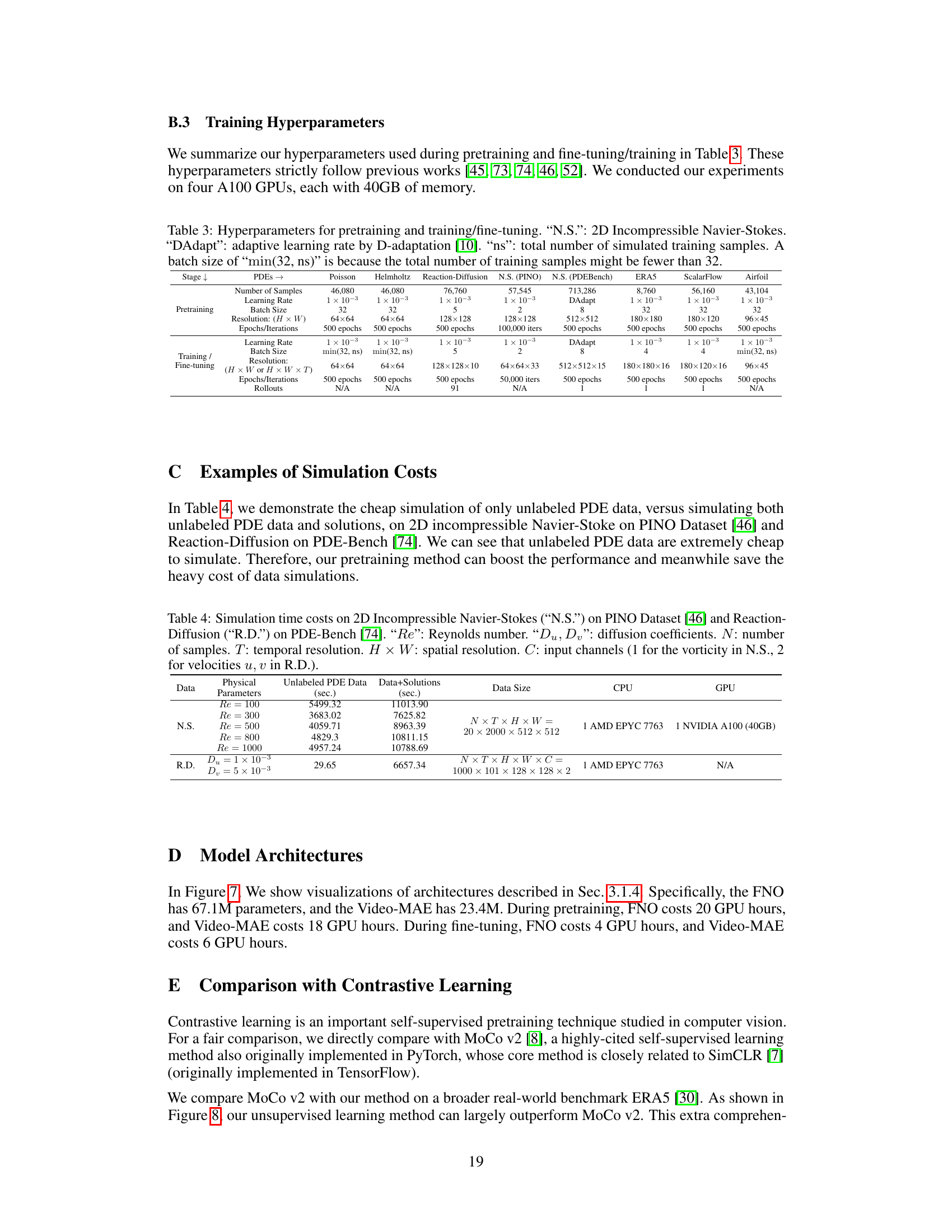
Table 3: Hyperparameters for pretraining and training/fine-tuning. “N.S.”: 2D Incompressible Navier-Stokes. 'DAdapt': adaptive learning rate by D-adaptation [10]. 'ns': total number of simulated training samples. A batch size of 'min(32, ns)' is because the total number of training samples might be fewer than 32.

🔼 This table compares the computation time required to generate unlabeled PDE data only versus generating both unlabeled data and solutions for two different PDEs: 2D incompressible Navier-Stokes and Reaction-Diffusion. It highlights the significant cost savings achievable by using only unlabeled data for unsupervised pretraining, making the approach more computationally feasible.
read the caption
Table 4: Simulation time costs on 2D Incompressible Navier-Stokes ('N.S.') on PINO Dataset [46] and Reaction-Diffusion ('R.D.') on PDE-Bench [74]. 'Re': Reynolds number. 'Du, Dv': diffusion coefficients. N: number of samples. T: temporal resolution. H × W: spatial resolution. C: input channels (1 for the vorticity in N.S., 2 for velocities u, v in R.D.).
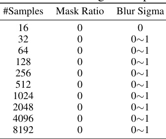
🔼 This table shows the best hyperparameter choices for mask ratio and blur sigma used during the pretraining phase of the Poisson equation, categorized by the number of training samples. The optimal values for these hyperparameters depend on the amount of data available.
read the caption
Table 5: Best choice of mask ratio and blur sigma for pretraining on Poisson equation.
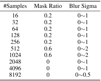
🔼 This table shows the best hyperparameter settings for the Helmholtz equation in the context of unsupervised pretraining. The hyperparameters considered are the mask ratio (portion of input data masked) and blur sigma (standard deviation of the Gaussian blur applied to the masked regions). The table demonstrates that the optimal hyperparameters depend on the amount of training data available.
read the caption
Table 6: Best choice of mask ratio and blur sigma for pretraining on Helmholtz equation.

🔼 This table shows the best hyperparameter settings (mask ratio and blur sigma) for pretraining a 2D Diffusion-Reaction equation model using different numbers of training samples. The optimal settings vary depending on the dataset size, suggesting that stronger perturbations (higher masking ratio and blur sigma) are beneficial when training data is scarce, while milder perturbations suffice with larger datasets.
read the caption
Table 7: Best choice of mask ratio and blur sigma for pretraining on 2D Diffusion-Reaction equation.
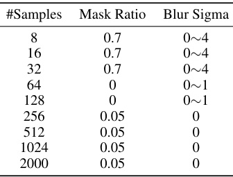
🔼 This table shows the best hyperparameter choices for mask ratio and blur sigma during the pretraining phase on the 2D incompressible Navier-Stokes equation, categorized by the number of training samples. It demonstrates that the optimal hyperparameters depend on the amount of data available.
read the caption
Table 8: Best choice of mask ratio and blur sigma for pretraining on 2D incompressible Navier-Stokes.

🔼 This table shows the impact of the number of unlabeled PDE data samples used for pretraining on the relative l2 error of the FNO model for the 2D incompressible Navier-Stokes equation. It demonstrates that increasing the number of pretraining samples leads to a reduction in the relative l2 error, suggesting that more data improves the quality of the pretrained model.
read the caption
Table 9: More unlabeled PDE data improve the quality of pretraining. FNO on 2D incompressible Navier-Stokes, pretrained with mask ratio as 0.7.
Full paper#

