TL;DR#
Many real-world phenomena are governed by underlying dynamical systems, but identifying the governing parameters from raw data is challenging. Existing causal representation learning (CRL) methods offer identifiability guarantees, but lack scalability; conversely, dynamical system methods are scalable but lack identifiability. This creates a critical need for methods that combine both strengths.
This research proposes a novel framework to address these limitations by bridging causal representation learning and dynamical systems. It demonstrates how parameter estimation problems in dynamical systems can be reformulated as latent variable identification problems in CRL. The proposed framework leverages scalable solvers for differential equations to build identifiable and practical models, allowing for out-of-distribution classification and treatment effect estimation. The efficacy of this approach is validated through experiments using a wind simulator and real-world climate data.
Key Takeaways#
Why does it matter?#
This paper is crucial because it bridges the gap between causal representation learning and dynamical systems, two seemingly disparate fields. By establishing this connection, researchers gain access to novel methods for identifying underlying physical parameters from real-world data, significantly advancing scientific understanding and practical applications.
Visual Insights#
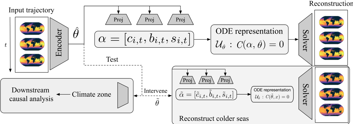
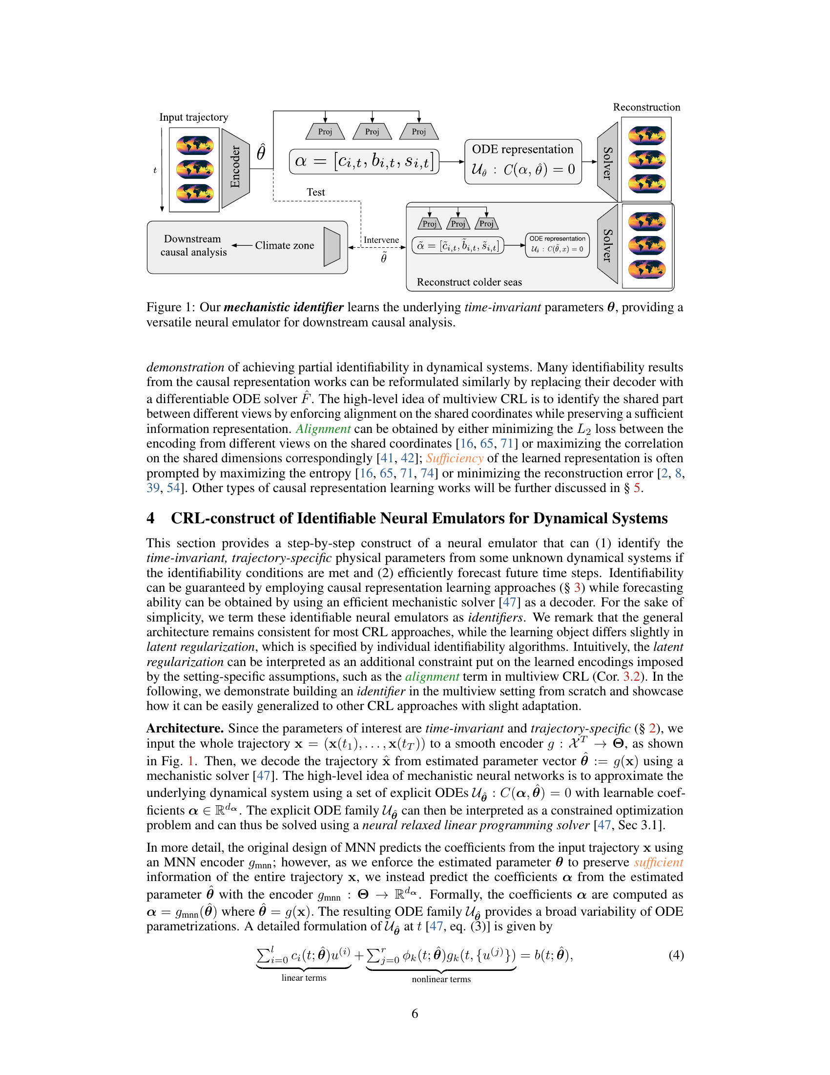
🔼 This figure illustrates the architecture of the proposed ‘mechanistic identifier,’ a neural network designed for identifying time-invariant physical parameters (θ) from real-world time-series data and using these parameters for downstream causal analysis. The input is a complete trajectory of the system’s state (represented as a sequence of maps of the globe). This trajectory is passed to an encoder that extracts a representation of the time-invariant parameters. A mechanistic neural network (MNN) solver is then used to decode the parameters back into a representation of the trajectory. The figure also highlights how interventions can be performed to understand the causal effect of specific parameters on the system. By manipulating the estimated parameter (θ) and feeding it back into the MNN, the model generates a modified trajectory. This allows the analysis of the causal impact of changing specific parameters, such as reconstructing ‘colder seas’ by adjusting a related parameter.
read the caption
Figure 1: Our mechanistic identifier learns the underlying time-invariant parameters θ, providing a versatile neural emulator for downstream causal analysis.

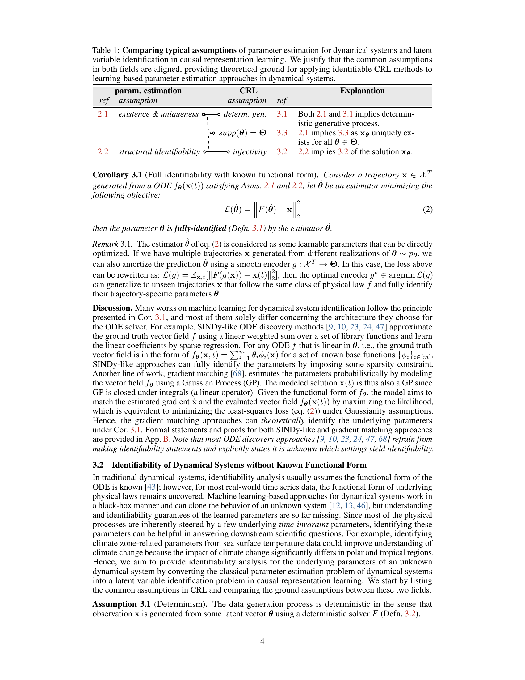
🔼 This table compares the assumptions made in parameter estimation for dynamical systems and latent variable identification in causal representation learning. The authors demonstrate that the common assumptions in both fields are aligned, providing a theoretical justification for applying identifiable causal representation learning (CRL) methods to parameter estimation problems in dynamical systems. This table highlights the connections between the two fields, facilitating the application of CRL techniques to improve the accuracy and reliability of parameter identification in dynamical systems.
read the caption
Table 1: Comparing typical assumptions of parameter estimation for dynamical systems and latent variable identification in causal representation learning. We justify that the common assumptions in both fields are aligned, providing theoretical ground for applying identifiable CRL methods to learning-based parameter estimation approaches in dynamical systems.
In-depth insights#
Causal Id. in Dynamics#
The heading ‘Causal Id. in Dynamics’ suggests an investigation into the intersection of causality and dynamical systems. The core idea likely revolves around identifying causal relationships within systems that evolve over time. This is a significant challenge because dynamical systems often involve complex interactions between multiple variables, making it difficult to disentangle cause and effect. The work probably explores methods to infer causal structures from observational data, potentially leveraging techniques from causal inference and machine learning. A key aspect might be the development or application of algorithms capable of identifying causal mechanisms underlying the observed dynamics, going beyond simple correlation. Identifiability— the ability to uniquely determine causal effects from data—is a crucial consideration, as is the handling of confounding factors which might obscure true causal relations. The research likely evaluates the performance of these methods on both synthetic and real-world datasets, potentially focusing on the interpretability of the results and their implications for understanding and predicting system behavior. Overall, the research aims to advance the application of causal reasoning to complex dynamical systems, offering a more robust way to analyze and understand these systems beyond mere correlation analysis.
Mech. Id. Framework#
A mechanistic identifier framework, as the name suggests, is designed to identify the underlying physical mechanisms of a system. It leverages causal representation learning principles to achieve this identifiability, contrasting with traditional approaches that often lack explicit guarantees. The core of the framework lies in combining a mechanistic neural network (MNN) ODE solver with a causal representation learning encoder. The encoder processes the input data to estimate time-invariant system parameters, and the MNN-ODE solver uses these estimates to reconstruct the system’s trajectory. This approach is particularly powerful for real-world applications where the underlying functional form of the system’s dynamics is unknown. Importantly, the framework can handle parameter estimation problems by recasting them as latent variable identification problems, directly benefiting from the established identifiability theory. This framework is evaluated on simulated and real-world datasets, demonstrating improved performance in downstream tasks such as out-of-distribution classification and treatment effect estimation. The framework offers a practical and theoretically grounded method for learning identifiable neural emulators of dynamical systems, opening up new possibilities in the analysis of complex systems across various scientific domains.
CRL-MNN Hybrid#
A CRL-MNN hybrid approach integrates causal representation learning (CRL) with mechanistic neural networks (MNNs) to identify and forecast in dynamical systems. CRL provides identifiability guarantees, ensuring that learned parameters correspond to true underlying physical mechanisms. MNNs offer efficient forecasting, leveraging differentiable solvers for differential equations. This combination overcomes limitations of traditional methods that either lack identifiability or struggle with scalability in complex systems. The hybrid model learns explicitly controllable models, isolating trajectory-specific parameters. This facilitates downstream tasks like out-of-distribution classification and causal effect estimation. The synergistic approach is particularly valuable for real-world applications where complex systems are involved, as it allows learning both accurate and interpretable models with reliable forecasts.
Climate Data Analysis#
Analyzing climate data involves understanding the complexities of long-term climate trends and variability. Key aspects include identifying patterns, such as temperature fluctuations, precipitation changes, and extreme weather events. Sophisticated statistical methods are crucial for analyzing noisy, incomplete, and spatially heterogeneous climate datasets. Advanced techniques, such as machine learning and causal inference, are increasingly used to detect subtle relationships, predict future changes, and unravel complex cause-and-effect mechanisms. Data visualization is essential for communicating findings effectively and conveying the impacts of climate change. Combining observational data with climate model simulations allows for a more comprehensive understanding of climate systems and the effects of human activity. This is essential for informing effective climate policy and adaptation strategies. Uncertainty quantification is crucial due to the inherent variability and complexity of climate data. This involves both understanding inherent dataset uncertainties and representing uncertainty within modeling techniques.
Future Research#
Future research directions stemming from this work are multifaceted. Extending the framework to handle stochastic differential equations (SDEs), rather than solely deterministic ODEs, is crucial for increased realism in modeling many real-world phenomena. Furthermore, explicitly incorporating measurement noise into the theoretical framework will enhance its robustness and applicability to real-world datasets plagued by inherent uncertainties. The current infinite data assumption is a limitation; future work should investigate finite-sample identifiability to make the approach more practical. Finally, exploring the synergistic potential of combining this work with other causal representation learning techniques, such as those employing multi-environment setups or temporal causal modeling, could unlock novel identifiable neural emulators with enhanced performance and broader applicability.
More visual insights#
More on figures

🔼 This figure illustrates the architecture of the proposed mechanistic identifier model. The model takes an input trajectory, encodes it into a latent representation of time-invariant parameters, and then uses these parameters to reconstruct the trajectory using a mechanistic solver, which approximates the underlying dynamical system. The time-invariant parameters are used for downstream causal analysis, such as out-of-distribution classification or treatment effect estimation. The figure highlights the key components of the model: the encoder, the mechanistic solver, and the downstream causal analysis tasks.
read the caption
Figure 1: Our mechanistic identifier learns the underlying time-invariant parameters θ, providing a versatile neural emulator for downstream causal analysis.
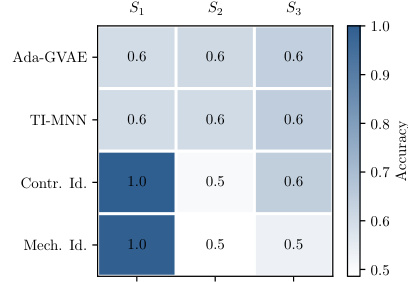
🔼 This figure shows the prediction accuracy of the layer thickness parameter in a wind simulation experiment. The model’s learned representation is split into three partitions (S1, S2, S3), each encoding different aspects of the data. The accuracy is evaluated separately for each partition. The results demonstrate the model’s ability to successfully identify the layer thickness parameter. Specifically, high accuracy is observed for partition S1, suggesting this part captures the target information efficiently, while lower accuracy in other partitions indicates they might capture less relevant information for this task.
read the caption
Figure 3: Prediction accuracy on layer thickness parameter on wind simulation data, evaluated on individual encoding partitions S1, S2, S3. Results averaged from three random runs.

🔼 The figure illustrates the architecture of the proposed ‘mechanistic identifier.’ It’s a neural network model that learns underlying time-invariant physical parameters (θ) from input trajectories. These parameters are crucial for understanding the underlying dynamical system. The model uses an encoder to extract information from the input trajectory, subsequently feeding this information into an ODE (Ordinary Differential Equation) representation, solved by a mechanistic solver. The output is then used for downstream causal analysis, including tasks like OOD classification and treatment-effect estimation.
read the caption
Figure 1: Our mechanistic identifier learns the underlying time-invariant parameters θ, providing a versatile neural emulator for downstream causal analysis.
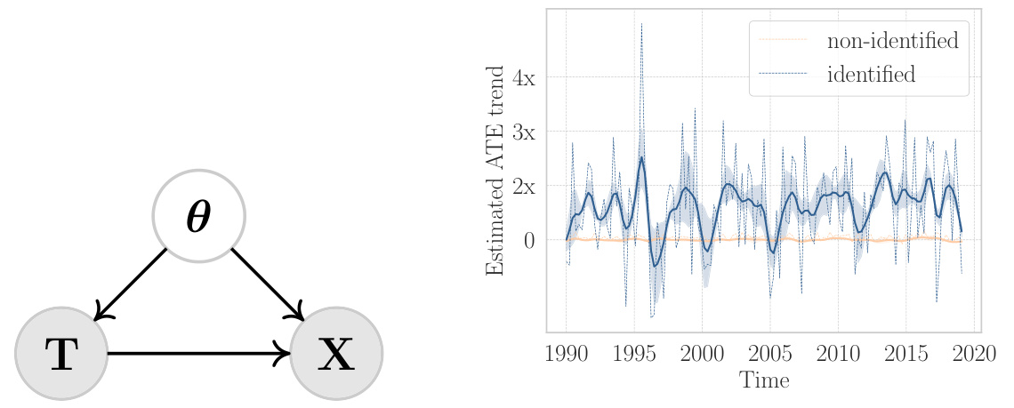
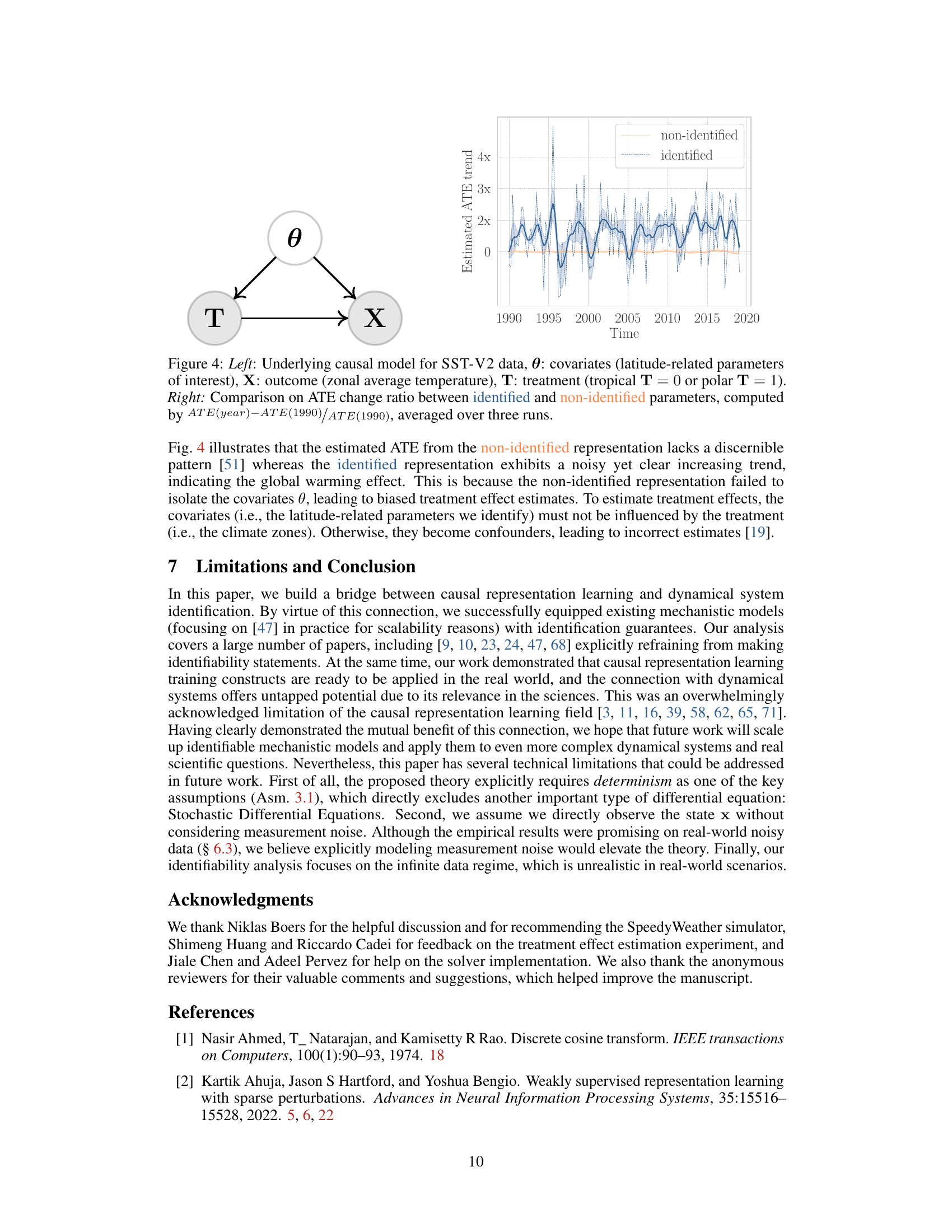
🔼 The figure shows a causal model and a comparison of results for estimating the average treatment effect (ATE) using identified and non-identified parameters on sea surface temperature data. The causal model (left panel) illustrates the relationship between latitude-related parameters (θ), climate zones (T), and zonal average temperature (X). The right panel shows that using identified parameters leads to a clearer increasing trend in ATE over time, reflecting global warming, while using non-identified parameters results in a less clear and more erratic trend.
read the caption
Figure 4: Left: Underlying causal model for SST-V2 data, θ: covariates (latitude-related parameters of interest), X: outcome (zonal average temperature), T: treatment (tropical T = 0 or polar T = 1). Right: Comparison on ATE change ratio between identified and non-identified parameters, computed by ATE(year)-ATE(1990)/ATE(1990), averaged over three runs.

🔼 The figure illustrates the architecture of the proposed mechanistic identifier. It consists of an encoder that takes an input trajectory and outputs time-invariant parameters. These parameters are then used by a mechanistic neural network (MNN) solver to reconstruct the trajectory, which can be used for downstream causal analysis tasks. The figure also shows the relationship between the learned representations and the downstream causal tasks.
read the caption
Figure 1: Our mechanistic identifier learns the underlying time-invariant parameters θ, providing a versatile neural emulator for downstream causal analysis.

🔼 The figure illustrates the architecture of the proposed mechanistic identifier, which combines causal representation learning with dynamical systems. It takes an input trajectory, encodes it to extract time-invariant parameters (θ), and then uses a mechanistic neural network (MNN) to reconstruct the trajectory. This process allows for downstream causal analysis tasks such as OOD classification or treatment effect estimation, based on the learned parameters. The identifier is trained using multi-view causal representation learning, which enables the identification of shared parameters between multiple trajectories.
read the caption
Figure 1: Our mechanistic identifier learns the underlying time-invariant parameters θ, providing a versatile neural emulator for downstream causal analysis.

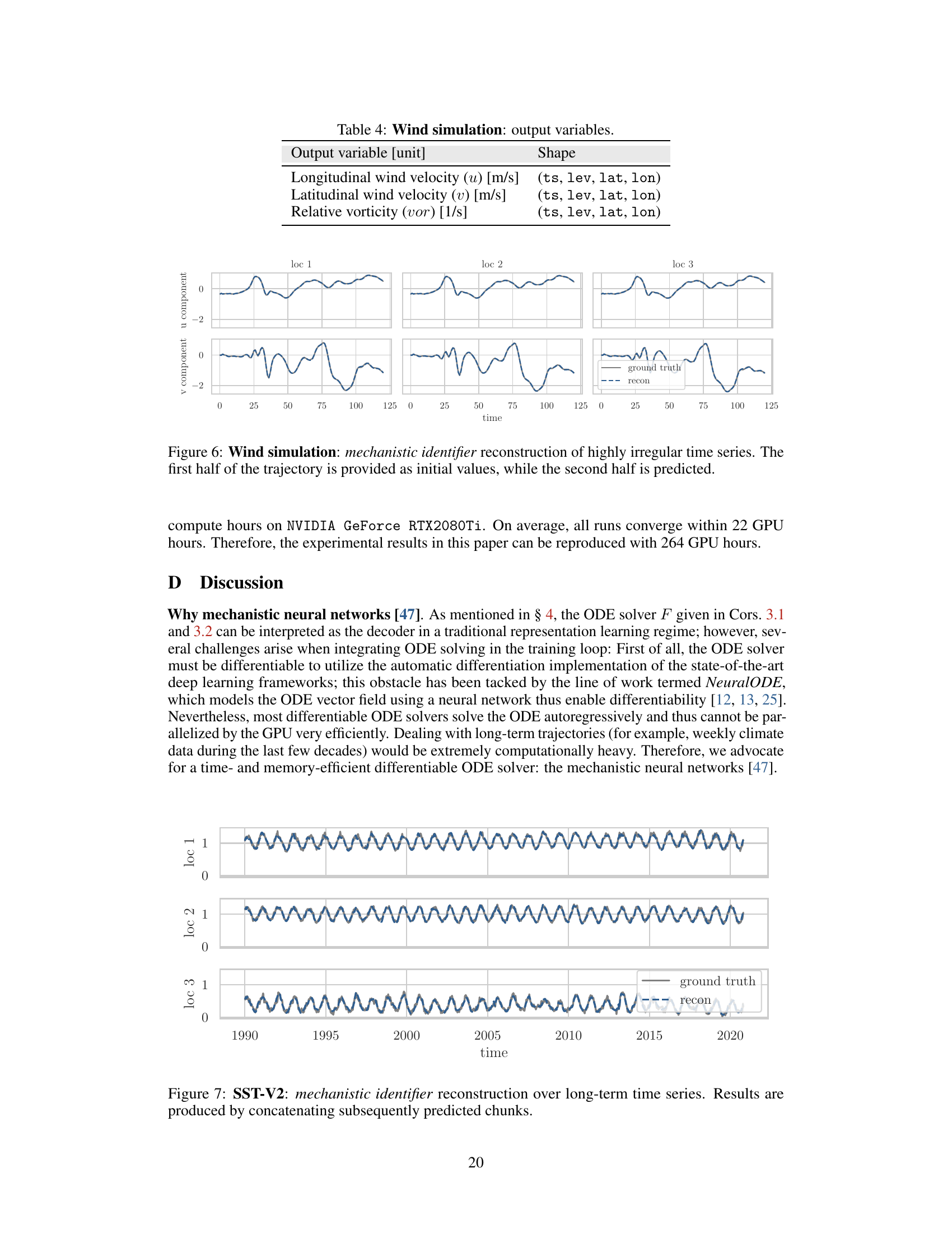
🔼 The figure shows the results of using a mechanistic identifier to reconstruct long-term time series data from the SST-V2 dataset. Three different locations (loc 1, loc 2, loc 3) are shown, each with the ground truth time series in gray and the reconstruction from the model in blue. The reconstructions are generated by concatenating shorter predictions made by the model, highlighting the model’s ability to forecast over longer time horizons. The quality of the reconstruction varies somewhat across the locations.
read the caption
Figure 7: SST-V2: mechanistic identifier reconstruction over long-term time series. Results are produced by concatenating subsequently predicted chunks.

🔼 This figure illustrates the architecture of the proposed ‘mechanistic identifier.’ The identifier takes an input trajectory (e.g., time series data) and uses an encoder to learn a representation that isolates the time-invariant, trajectory-specific physical parameters (θ). These parameters are then used to drive a mechanistic ODE solver, which produces a reconstructed trajectory. This reconstructed trajectory can then be used for various downstream causal analysis tasks, such as out-of-distribution classification or treatment effect estimation. The figure highlights the key components: the input trajectory, encoder, ODE representation (with parameters θ), solver, reconstruction, and downstream tasks. Importantly, the model is designed to be identifiable, meaning that the learned parameters accurately reflect the true underlying physical parameters, allowing for reliable causal inference.
read the caption
Figure 1: Our mechanistic identifier learns the underlying time-invariant parameters θ, providing a versatile neural emulator for downstream causal analysis.
More on tables

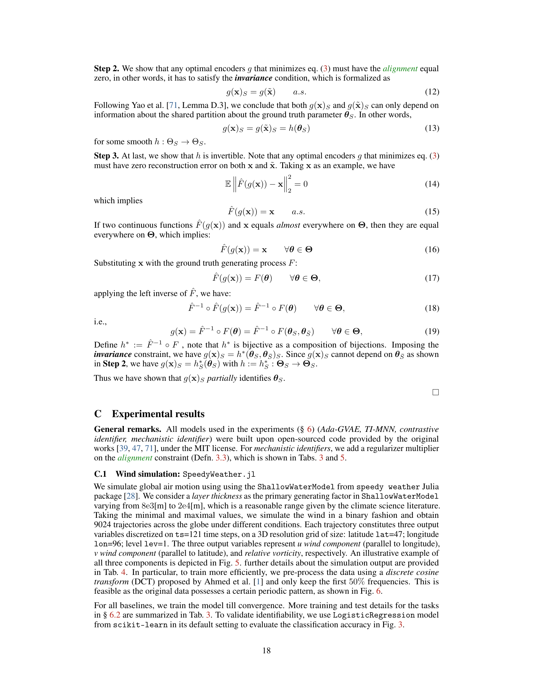
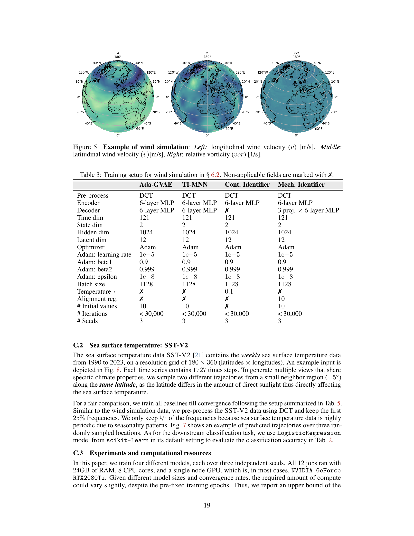
🔼 This table details the training setup used for the wind simulation experiment in section 6.2 of the paper. It compares four different models (Ada-GVAE, TI-MNN, Contrastive Identifier, and Mechanistic Identifier) across various hyperparameters including pre-processing techniques, encoder/decoder architecture, optimizer settings, and regularization parameters. The table highlights the differences in configurations for each model and indicates which parameters were not applicable (marked with ‘X’).
read the caption
Table 3: Training setup for wind simulation in § 6.2. Non-applicable fields are marked with X.

🔼 This table presents the results of validating Theorem 3.1, which states that parameters of ODEs with known functional forms are fully identifiable. The experiment uses 63 ODEs from the ODEBench dataset [15] and the Cart-Pole system [72]. For each ODE, 100 sets of parameters were randomly sampled, and the root mean square error (RMSE) between the estimated and true parameters was calculated. The RMSE is averaged across parameter dimensions and reported, along with standard deviations. The table demonstrates high accuracy in parameter estimation across various ODEs, supporting the theorem.
read the caption
Table 7: Theorem 3.1 validation using ODEs with known functional form: Experiments on complex dynamical systems from ODEBench [15] and Cart-Pole (inspired by Yao et al. [72]), for exact parameter identification. RMSE is computed over 100 randomly sampled parameter groups (nearby chaotic configuration for chaotic systems) and averaged over the parameter dimension.
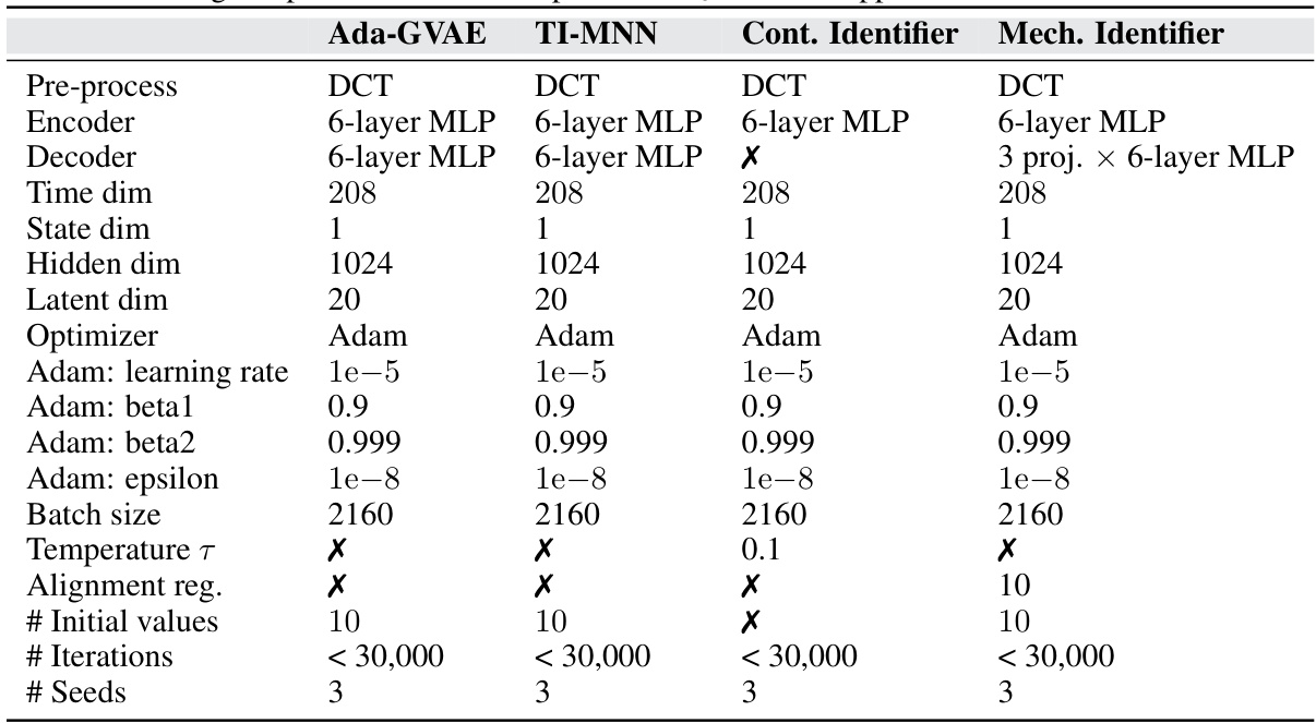
🔼 This table details the hyperparameters and settings used for training four different models (Ada-GVAE, TI-MNN, Contrastive Identifier, and Mech. Identifier) on the SST-V2 sea surface temperature dataset. It specifies pre-processing steps (DCT), encoder and decoder architectures (MLP layers), time and state dimensions of the data, hidden and latent dimensions of the models, optimization parameters (Adam optimizer settings), batch size, temperature (for contrastive learning), alignment regularization (for Mech. Identifier), the number of initial values, iterations, and the number of random seeds used for each model. Note that the Decoder and Alignment regularization are not used in all of the models.
read the caption
Table 5: Training setup for sea surface temperature in § 6.3. Non-applicable fields are marked with X.

🔼 This table compares the assumptions made in parameter estimation for dynamical systems and latent variable identification in causal representation learning. It shows that the common assumptions in both fields align, providing a theoretical basis for using identifiable causal representation learning (CRL) methods in parameter estimation for dynamical systems. The table highlights the connections between ’existence & uniqueness’, ‘structural identifiability’, and their counterparts in CRL, explaining how these shared assumptions justify the application of CRL techniques to improve parameter estimation in dynamical systems.
read the caption
Table 1: Comparing typical assumptions of parameter estimation for dynamical systems and latent variable identification in causal representation learning. We justify that the common assumptions in both fields are aligned, providing theoretical ground for applying identifiable CRL methods to learning-based parameter estimation approaches in dynamical systems.
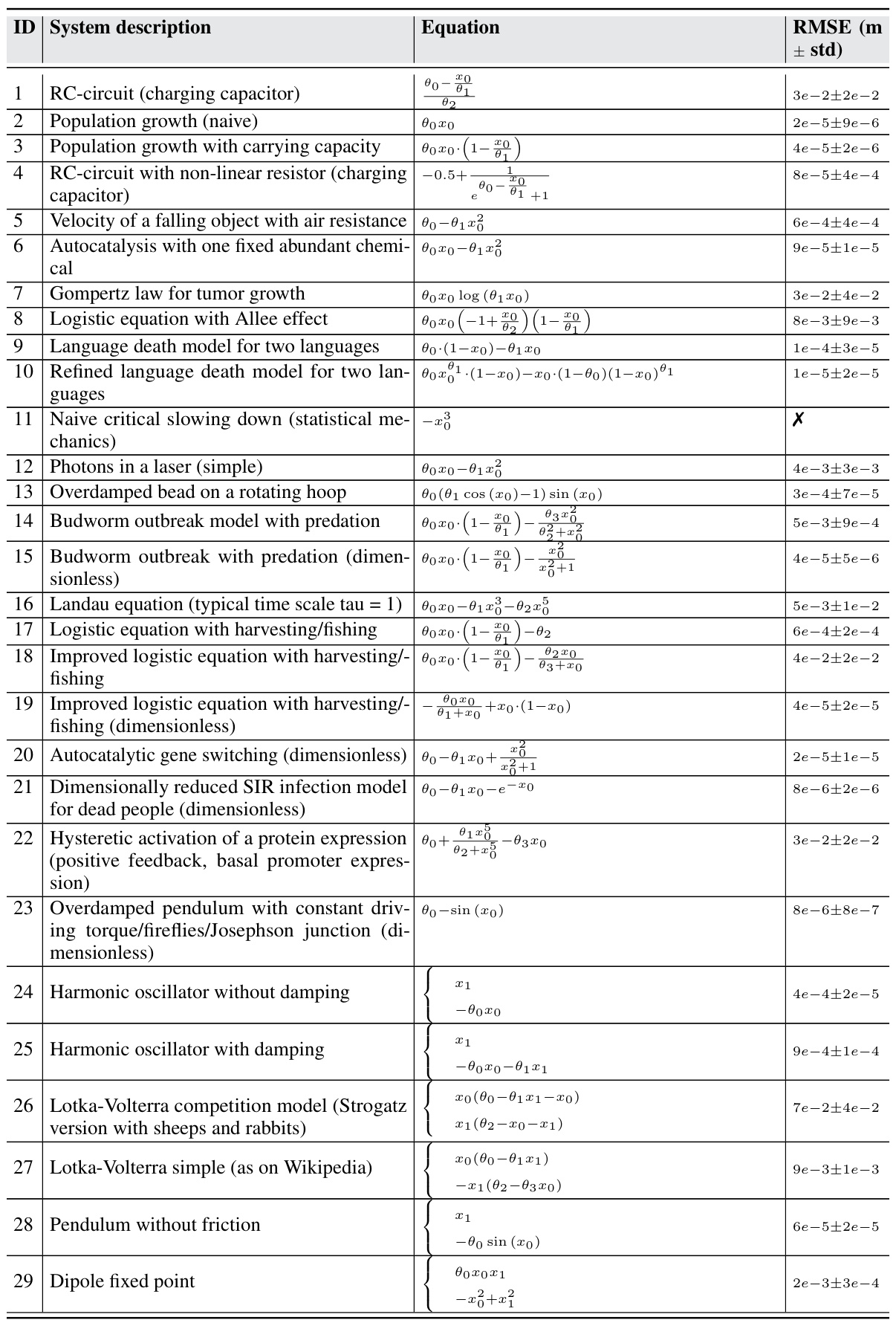
🔼 This table presents the results of validating Theorem 3.1, which states that parameters of ODEs with known functional forms are fully identifiable. The validation was done using 63 dynamical systems from the ODEBench dataset [15] and the Cart-Pole system [72]. For each system, 100 sets of parameters were randomly sampled, and the root mean square error (RMSE) between the estimated and true parameters was calculated. The table lists the system ID, description, equation, and the average RMSE across all parameters for each system.
read the caption
Table 7: Theorem 3.1 validation using ODEs with known functional form: Experiments on complex dynamical systems from ODEBench [15] and Cart-Pole (inspired by Yao et al. [72]), for exact parameter identification. RMSE is computed over 100 randomly sampled parameter groups (nearby chaotic configuration for chaotic systems) and averaged over the parameter dimension.

🔼 This table presents the results of validating Theorem 3.1, which concerns the full identifiability of parameters in ODEs with known functional forms. The experiment uses 63 dynamical systems from the ODEBench dataset [15] and the Cart-Pole system [72]. For each system, 100 sets of parameters were randomly sampled, and the root mean square error (RMSE) between the estimated and true parameters was calculated and averaged across all parameter dimensions. The table shows the system ID, a description of the system, the system’s equation, and the resulting RMSE values.
read the caption
Table 7: Theorem 3.1 validation using ODEs with known functional form: Experiments on complex dynamical systems from ODEBench [15] and Cart-Pole (inspired by Yao et al. [72]), for exact parameter identification. RMSE is computed over 100 randomly sampled parameter groups (nearby chaotic configuration for chaotic systems) and averaged over the parameter dimension.

🔼 This table presents the results of a validation experiment for Theorem 3.1, which concerns the full identifiability of parameters in ODEs with known functional forms. The experiment uses 63 dynamical systems from the ODEBench dataset [15], along with the Cart-Pole system (inspired by Yao et al. [72]). For each system, 100 sets of parameters were randomly sampled, and the root mean square error (RMSE) between the estimated and true parameters was calculated. The RMSE values are averaged over the parameter dimensions and reported along with their standard deviations, providing a quantitative assessment of the accuracy of parameter identification.
read the caption
Table 7: Theorem 3.1 validation using ODEs with known functional form: Experiments on complex dynamical systems from ODEBench [15] and Cart-Pole (inspired by Yao et al. [72]), for exact parameter identification. RMSE is computed over 100 randomly sampled parameter groups (nearby chaotic configuration for chaotic systems) and averaged over the parameter dimension.
Full paper#


