TL;DR#
Training large language models (LLMs) is computationally expensive, demanding significant memory and processing power. Existing methods like low-rank parameterization aim for efficiency but often compromise performance, especially during pretraining. Low-rank structures, while useful for fine-tuning, restrict parameters to a low-dimensional space and struggle to capture the full representation power needed for effective pretraining. This limitation hinders the ability to train larger and more complex models.
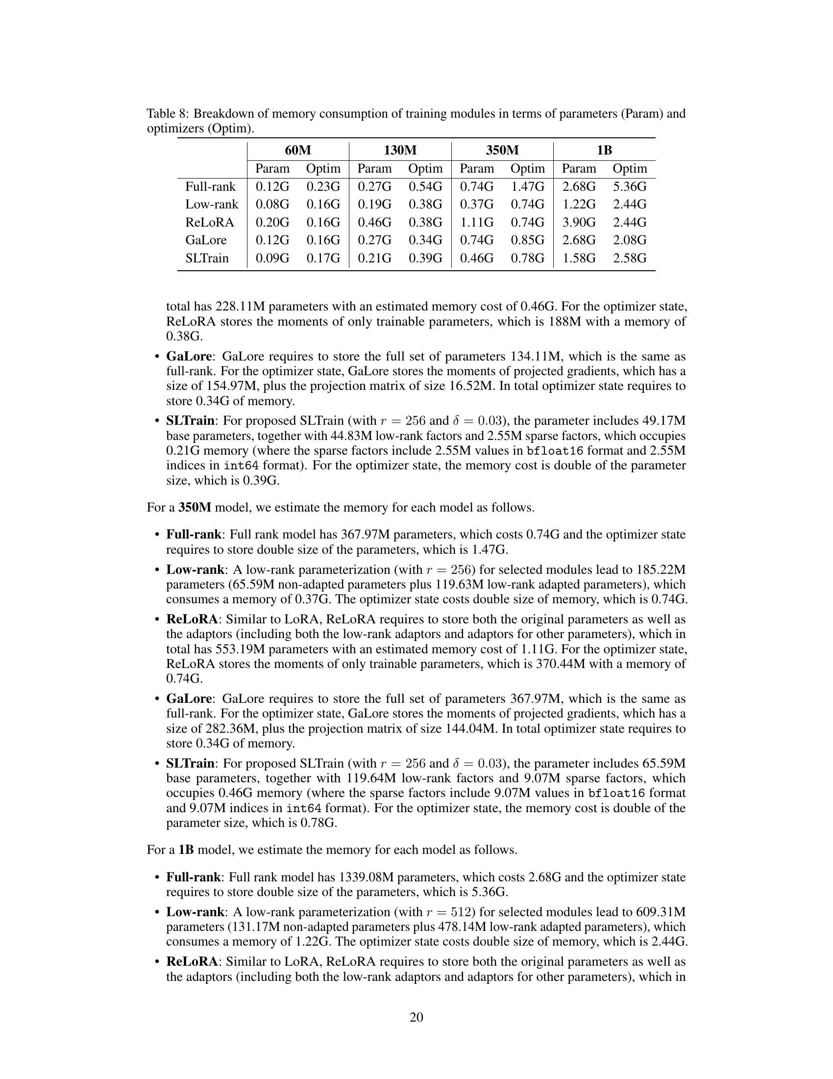
This paper introduces SLTrain, a novel approach that parameterizes the weights as a sum of low-rank and sparse matrices for pretraining. The low-rank component is learned through matrix factorization, while the sparse component utilizes a random, fixed-support learning strategy. This strategy, while simple, significantly improves pretraining efficiency. SLTrain achieves substantially better performance than low-rank pretraining while adding minimal extra parameters and memory costs. Combined with quantization and per-layer updates, it reduces memory requirements by up to 73% when pretraining LLaMA 7B model.
Key Takeaways#
Why does it matter?#
This paper is crucial for researchers working on large language models (LLMs) because it introduces a novel and efficient pretraining approach. SLTrain directly addresses the limitations of current low-rank methods by combining low-rank and sparse structures, resulting in significant improvements in parameter and memory efficiency without sacrificing performance. This opens new avenues for training even larger LLMs with limited resources, making it highly relevant to current research trends in the field.
Visual Insights#
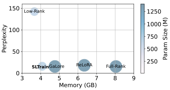
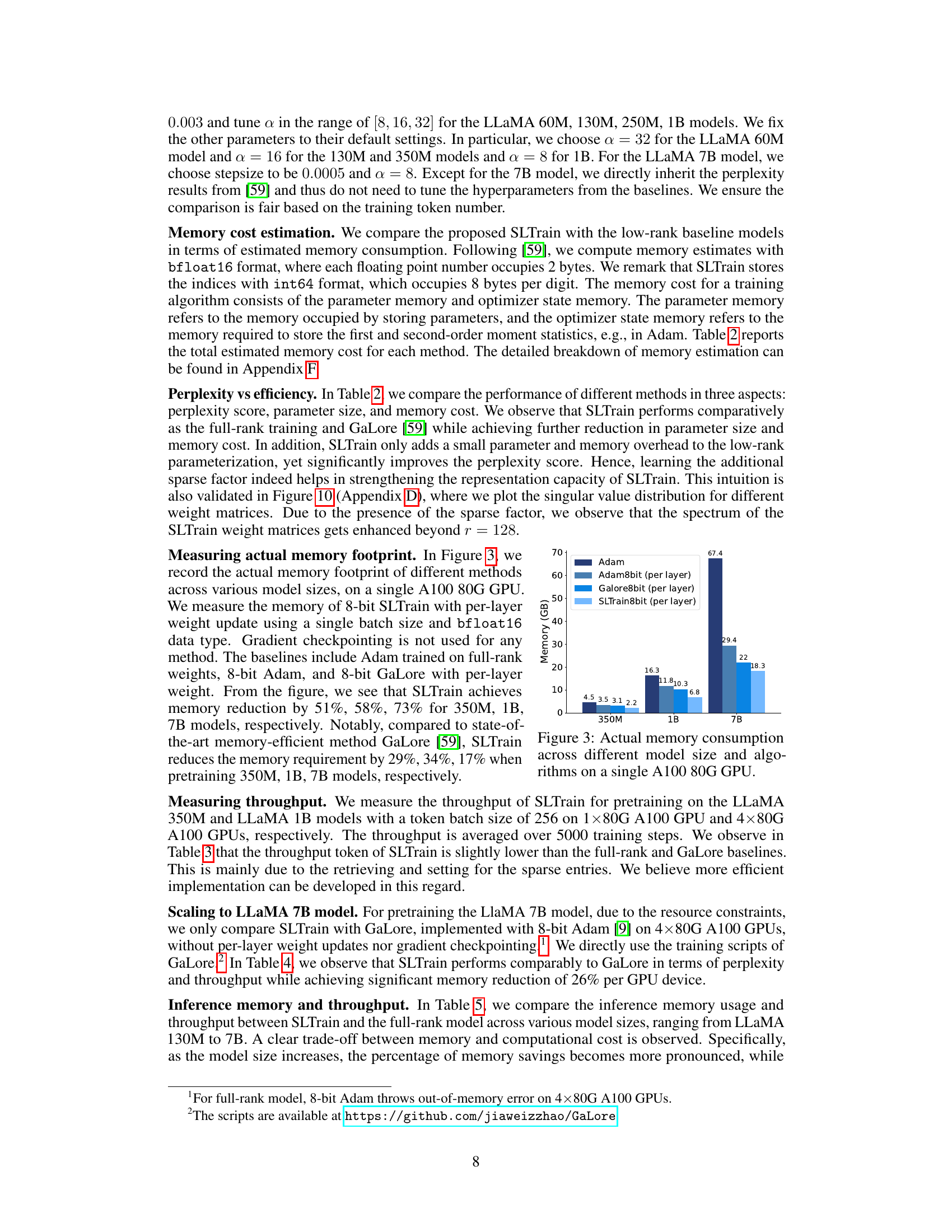
🔼 This figure compares several methods for pretraining the LLaMA 1B language model on the C4 dataset. The methods are represented by circles, with the size and color of each circle corresponding to the parameter size of the model. The vertical axis represents the model’s perplexity (a measure of how well the model predicts text), and the horizontal axis shows the memory usage. Methods that result in smaller, lighter circles are preferred since they provide good performance with reduced parameter and memory requirements. The figure highlights the trade-off between model size, memory, performance, and illustrates the advantages of SLTrain (a method proposed in the paper).
read the caption
Figure 1: Shown are perplexity, memory, and parameter size for pretraining LLaMA 1B on the C4 dataset with different methods. The radius and color of each circle scale with parameter size. Overall, the methods which have smaller, lighter circles on the left bottom corner are desirable for pretraining. The details are in Section 5.1.
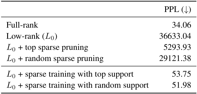
🔼 The table presents the perplexity scores (PPL) achieved using different training and pruning methods on the LLaMA 60M language model trained on 1.1B tokens. It compares the full-rank model with low-rank approximations (Lo) and further experiments that combine low-rank with different sparse pruning and training strategies. Notably, it highlights that using random sparse support for training is comparable to using top sparse support, motivating the use of random fixed-support sparse learning combined with low-rank learning in SLTrain.
read the caption
Table 1: Perplexity (PPL) of training and pruning with random versus top sparsity for LLaMA 60M on 1.1B tokens.
In-depth insights#
Low-Rank Limits#
The concept of ‘Low-Rank Limits’ in the context of large language model (LLM) training refers to the inherent constraints imposed when using low-rank approximations of the model’s weight matrices. While low-rank methods offer significant advantages in terms of reduced computational cost and memory footprint, they also restrict the model’s representational capacity. This limitation arises because low-rank matrices inherently lie in a lower-dimensional subspace compared to full-rank matrices. Therefore, the expressiveness of the model is inevitably curtailed, leading to a potential trade-off between efficiency and performance. This trade-off is a central challenge in the pursuit of efficient LLM training. Approaches like the addition of sparse components, as suggested in the research paper, may alleviate some of these limitations by enhancing the model’s capacity to capture complex relationships without significantly increasing computational demand. Understanding these limitations is key to designing effective strategies for efficient, yet high-performing LLMs. Future research may focus on adaptive low-rank techniques that dynamically adjust the rank based on the training data and task demands, thereby mitigating the limitations of static low-rank parameterizations.
Sparse Plus LR#
The concept of “Sparse Plus Low-Rank” (LR) represents a hybrid approach to parameter-efficient model training, combining the strengths of both sparse and low-rank matrix factorizations. Sparsity reduces the number of parameters directly by setting many weights to zero. This offers significant memory savings and computational efficiency, particularly beneficial for large language models. Low-rank factorization approximates a full-rank weight matrix using the product of two smaller matrices, reducing the number of parameters required to represent the model. This also leads to faster training and inference speeds. By combining these two techniques, the “Sparse Plus LR” approach aims to capture the most important information in the weight matrices concisely and efficiently. This involves identifying the most influential weights (low-rank component) while also eliminating less important ones (sparse component). The method’s effectiveness hinges on a careful balance: too much sparsity risks loss of information crucial for model accuracy, while insufficient sparsity negates the memory benefits. Similarly, a low-rank approximation that is too low may underfit the data, compromising performance. A key research question would be how to optimally determine the degree of sparsity and the rank to ensure an appropriate trade-off between model size and accuracy. The random support selection strategy for sparse learning is intriguing; however, more sophisticated techniques might yield even greater improvements. The approach promises a significant reduction in the memory footprint required for both training and deploying large models.
SLTrain Method#
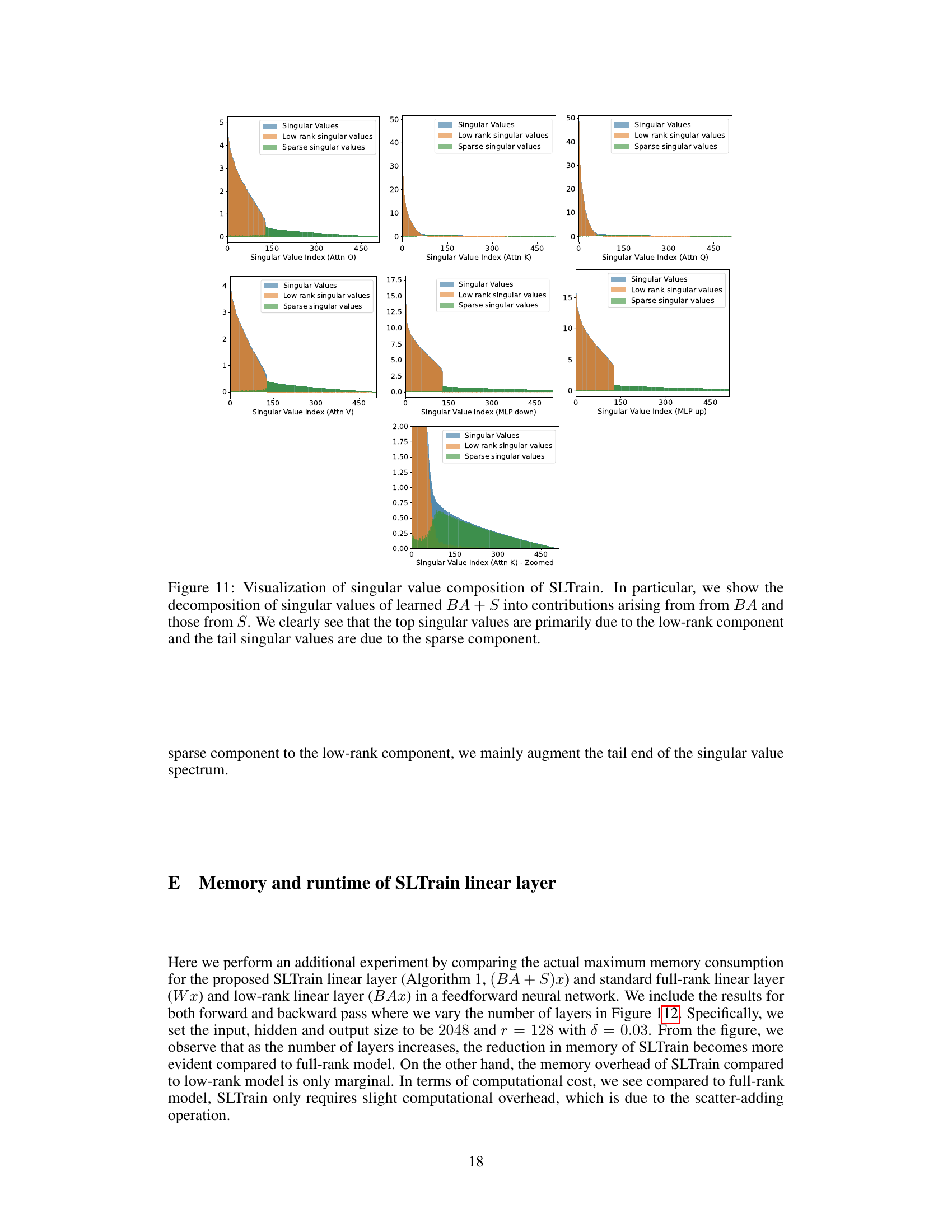
The core of the SLTrain method lies in its novel parameterization of weight matrices. Instead of using a standard full-rank representation, SLTrain cleverly decomposes each weight matrix into the sum of a low-rank component and a sparse component. This dual approach is key to achieving both parameter and memory efficiency. The low-rank component is learned through matrix factorization, effectively capturing dominant patterns in the data with a limited number of parameters. Simultaneously, the sparse component, using a randomly selected and fixed support, strategically identifies important neuron-wise interactions. This random fixed-support strategy is crucial, making SLTrain computationally efficient because it avoids complex iterative pruning and growth algorithms typically needed in sparse learning methods. The combination of low-rank and sparse components yields a pretrained model with high representational power while minimizing memory footprint. The strategy of optimizing only the non-zero values in the sparse component is a major innovation, significantly reducing memory demands compared to previous low-rank or sparse methods. SLTrain’s architecture allows for seamless integration with quantization and per-layer updates, maximizing memory savings.
Memory Gains#
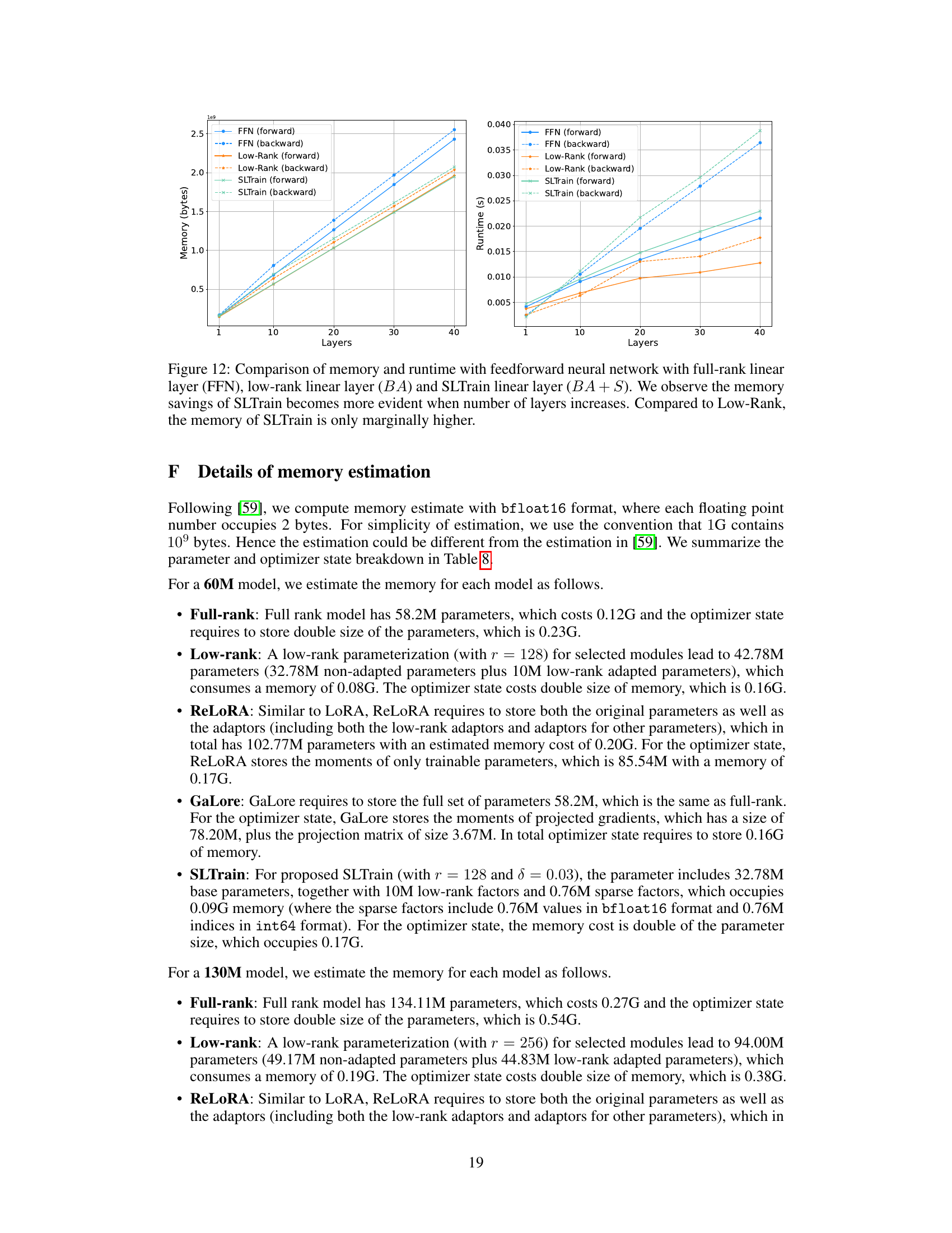
The concept of ‘Memory Gains’ in the context of large language model (LLM) training is crucial for practical application. Reducing memory footprint is paramount as it directly impacts the feasibility of training and deploying larger, more powerful LLMs. The paper explores memory efficiency through a combination of low-rank and sparse weight parameterization. SLTrain’s memory gains stem from two key factors: a reduction in the number of parameters and a novel strategy for handling the sparse component. The fixed-support sparse learning avoids the need to store a full sparse matrix, leading to substantial memory savings. Importantly, the memory reduction is achieved without significant performance degradation, often achieving performance comparable to full-rank training. Quantization and per-layer updates further amplify the memory gains, demonstrating a practical approach to train LLMs on more modest hardware resources. The effectiveness of the approach is demonstrated across varying LLM sizes, showing consistent improvements in memory efficiency without sacrificing model accuracy.
Future Works#
Future research directions stemming from this sparse plus low-rank approach for efficient LLM pretraining could involve several key areas. Improving the sparsity selection strategy beyond uniform random sampling is crucial; exploring adaptive or learned sparsity patterns could significantly enhance performance and efficiency. Investigating alternative low-rank factorization techniques and comparing them to the current approach would be valuable, potentially leading to more robust and effective model compression. A thorough theoretical analysis is needed to rigorously establish the convergence guarantees and generalization properties of the proposed method. Furthermore, extending the method to other large foundation models, beyond LLMs such as vision or multimodal models, is a promising avenue. Finally, combining SLTrain with other memory-efficient optimization techniques, such as quantization and gradient checkpointing, holds potential for even greater memory savings and scalability. Investigating the effects of different initialization strategies for the sparse and low-rank components warrants further study. Understanding the interplay between sparsity, rank, and model architecture to better determine the optimal hyperparameters could improve both the efficiency and performance.
More visual insights#
More on figures

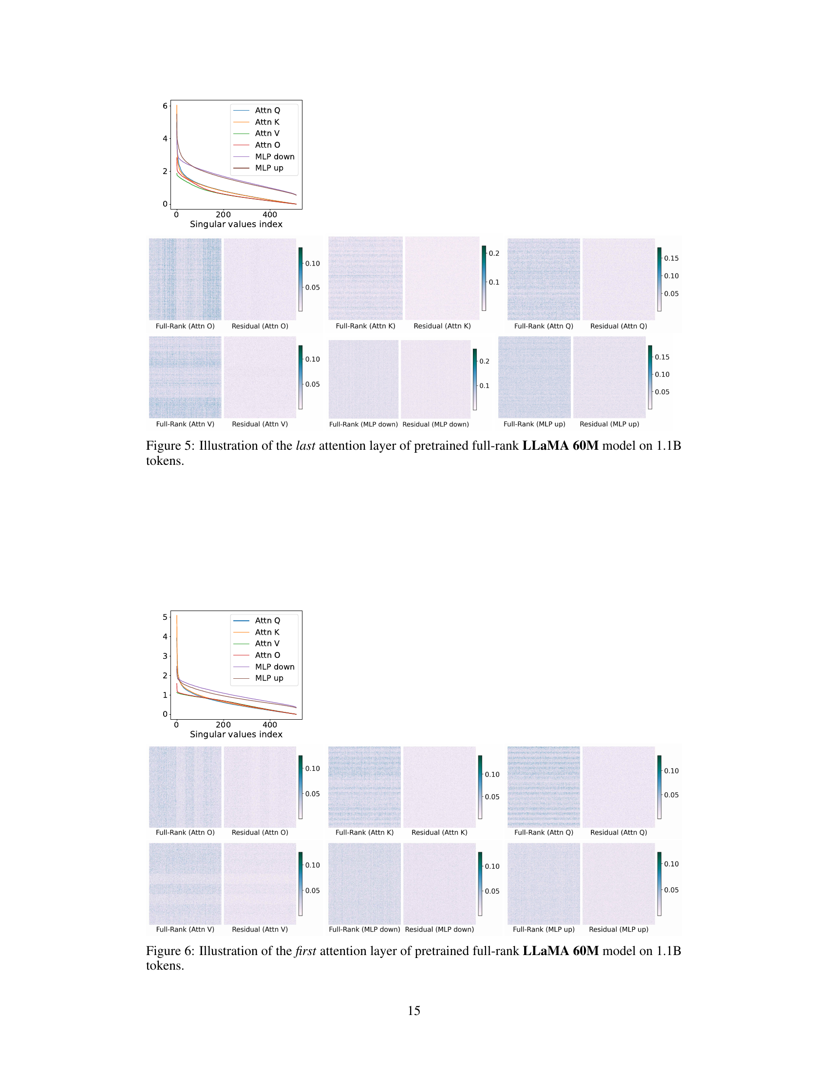
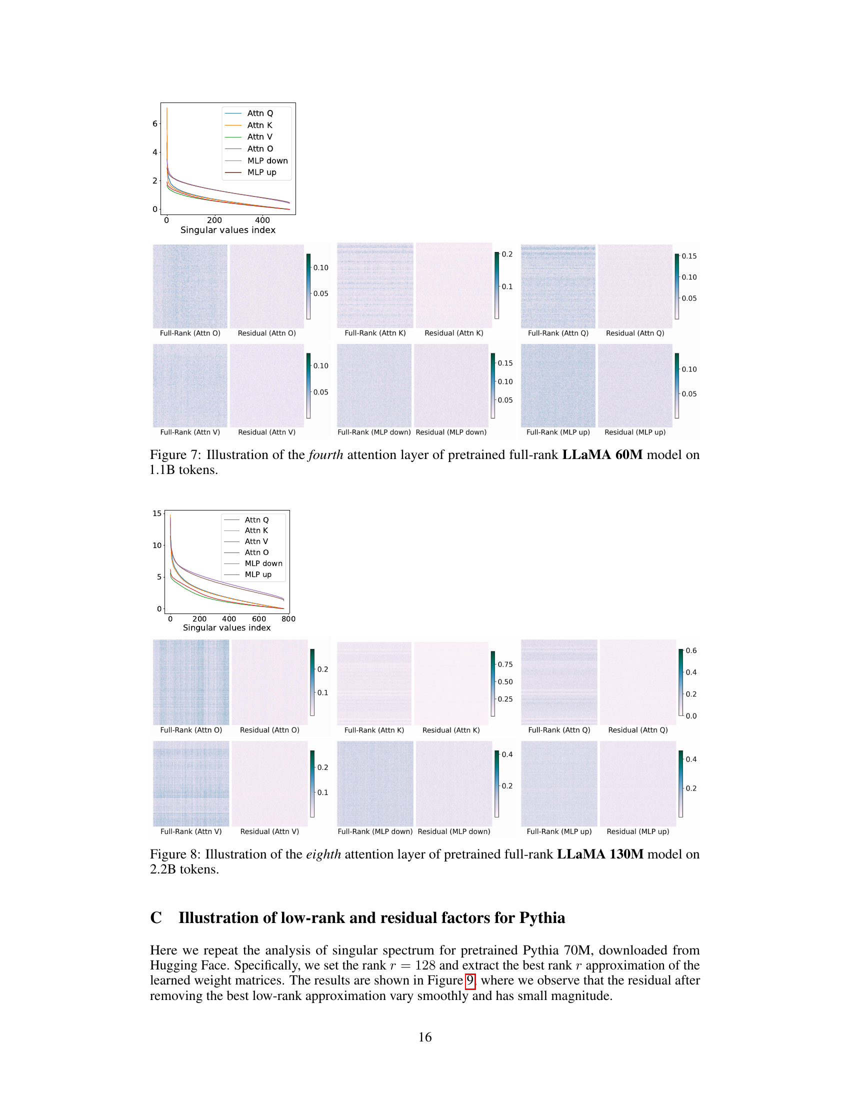
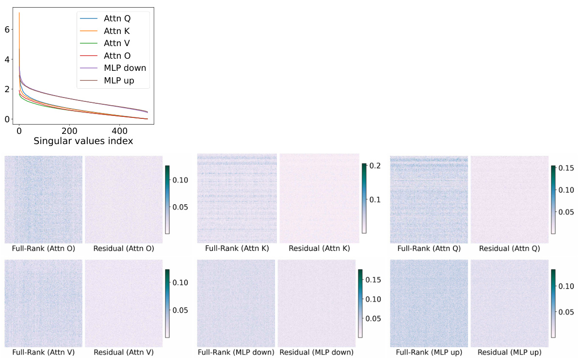
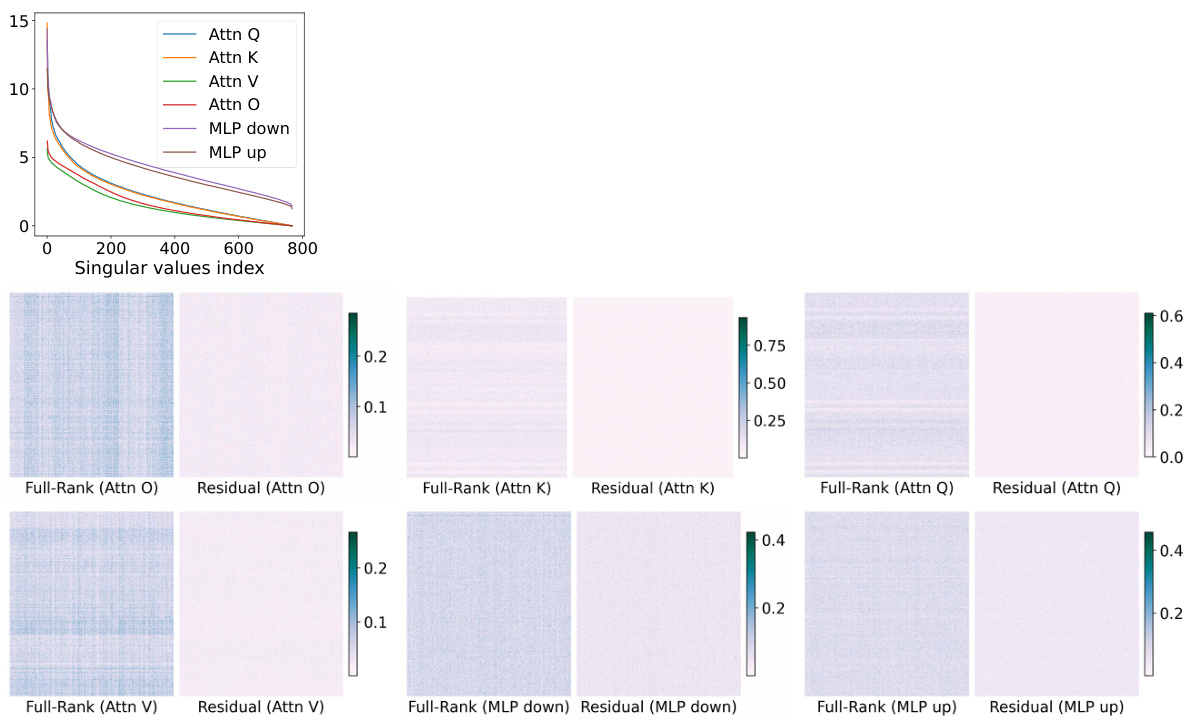
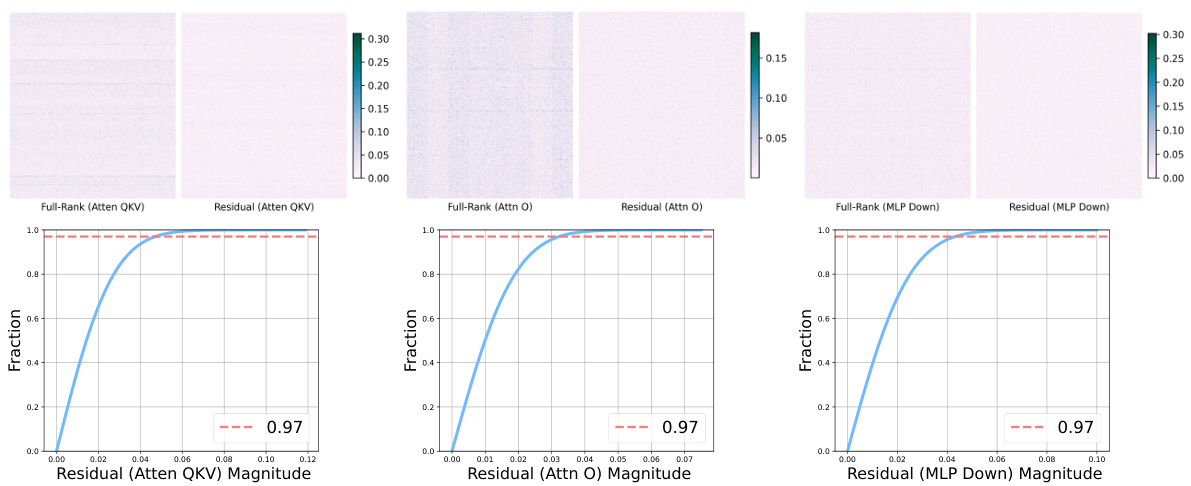
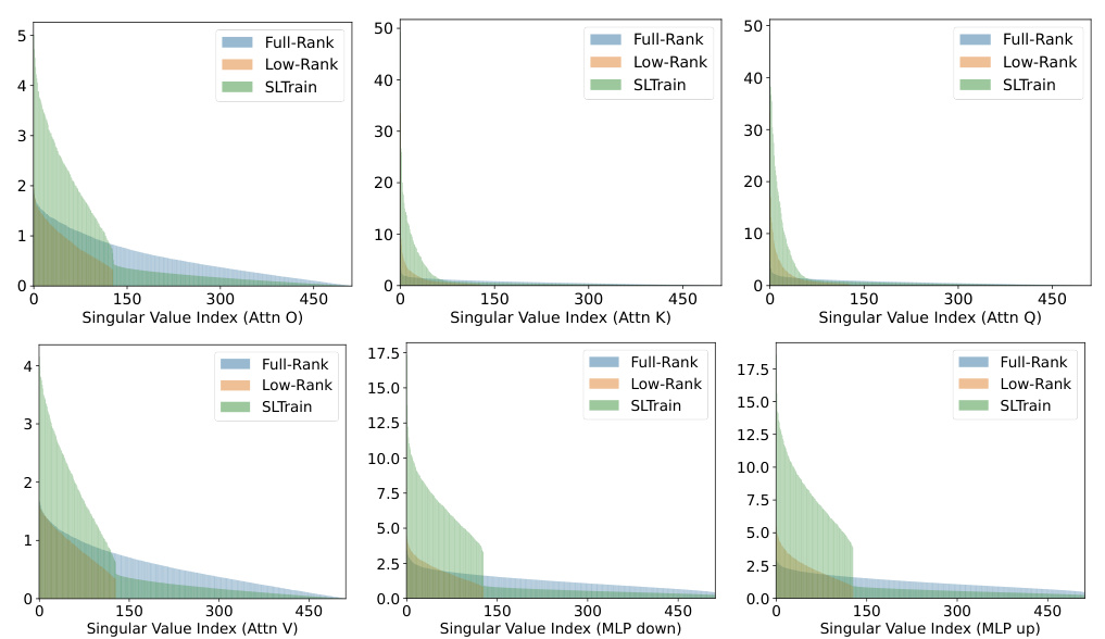
🔼 This figure provides an illustration of the weight matrices in the last attention layer of a pretrained LLaMA 60M model. It shows the singular value distribution (a), visualizes the full-rank matrix and its residual after low-rank approximation (b), and presents the cumulative density of the residual matrix magnitudes (c). The figure supports the argument for using sparse plus low-rank parameterization by demonstrating that a significant portion of the residual matrix has small magnitudes, suitable for sparse representation.
read the caption
Figure 2: Illustration of the last attention layer of pretrained full-rank LLaMA 60M model on 1.1B tokens. (a): singular value magnitudes of weight matrices where we observe a rapid decay of singular values. (b): Visualization of full-rank pretrained attention output matrix Wo in magnitude and the residual matrix after removing the best rank-r (r = 128) approximation of the Wo by SVD. We observe the magnitudes of the residual vary smoothly across different neuron-neuron interactions. (c): Cumulative density of the residual matrix in magnitude where we include a cut-off fraction at 0.97. We observe 97% entries in the residual matrix have magnitude less than 0.04.
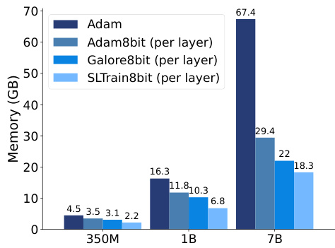
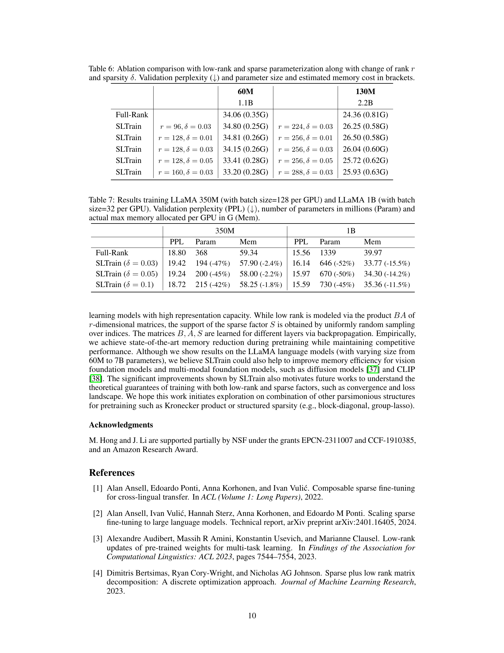
🔼 This figure shows the actual memory usage (in GB) of different training algorithms across various model sizes (350M, 1B, and 7B parameters) on a single NVIDIA A100 80GB GPU. The algorithms compared include full-rank Adam training, 8-bit Adam with per-layer updates, 8-bit GaLore with per-layer updates, and 8-bit SLTrain with per-layer updates. The bar chart visually represents the memory efficiency gains achieved by SLTrain compared to the other methods, especially as model size increases.
read the caption
Figure 3: Actual memory consumption across different model size and algorithms on a single A100 80G GPU.
🔼 This figure compares the performance of various LLM pretraining methods on the LLaMA 1B model using the C4 dataset. The methods are compared based on three metrics: perplexity, memory usage, and parameter size. Each method is represented by a circle where the size and color of the circle correspond to the parameter size. Methods with smaller, lighter circles, located in the lower-left corner (low perplexity, low memory, and low parameter size), are considered more desirable for efficient pretraining.
read the caption
Figure 1: Shown are perplexity, memory, and parameter size for pretraining LLaMA 1B on the C4 dataset with different methods. The radius and color of each circle scale with parameter size. Overall, the methods which have smaller, lighter circles on the left bottom corner are desirable for pretraining. The details are in Section 5.1.

🔼 This figure provides a visualization of the weight matrices in the last attention layer of a pretrained LLaMA 60M model. It shows the singular value distribution, which decays rapidly, indicating a low-rank structure. The visualization also shows the residual matrix after removing the best rank-128 approximation, highlighting that the remaining values are small and smoothly distributed. The cumulative density plot further emphasizes that most (97%) of these residual values are less than 0.04.
read the caption
Figure 2: Illustration of the last attention layer of pretrained full-rank LLaMA 60M model on 1.1B tokens. (a): singular value magnitudes of weight matrices where we observe a rapid decay of singular values. (b): Visualization of full-rank pretrained attention output matrix Wo in magnitude and the residual matrix after removing the best rank-r (r = 128) approximation of the Wo by SVD. We observe the magnitudes of the residual vary smoothly across different neuron-neuron interactions. (c): Cumulative density of the residual matrix in magnitude where we include a cut-off fraction at 0.97. We observe 97% entries in the residual matrix have magnitude less than 0.04.
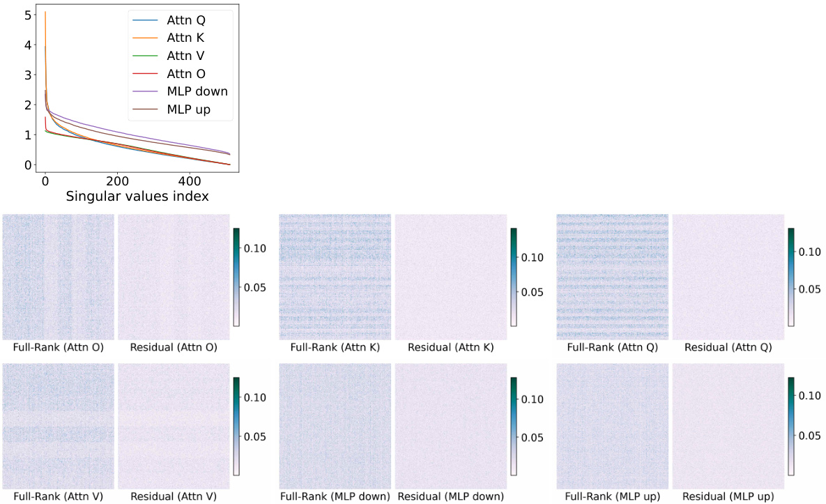
🔼 This figure shows the singular value distribution and visualization of the residual matrix in the last attention layer of a pretrained LLaMA 60M model. Subfigure (a) illustrates the rapid decay of singular values, demonstrating the potential for low-rank approximation. Subfigure (b) visualizes the magnitude of the full-rank attention output matrix and the residual after low-rank approximation, showing the smooth variation of residual entries. Subfigure (c) displays the cumulative density of the residual matrix, indicating that 97% of the entries have a magnitude less than 0.04, suggesting that a sparse matrix could effectively approximate the residual.
read the caption
Figure 2: Illustration of the last attention layer of pretrained full-rank LLaMA 60M model on 1.1B tokens. (a): singular value magnitudes of weight matrices where we observe a rapid decay of singular values. (b): Visualization of full-rank pretrained attention output matrix Wo in magnitude and the residual matrix after removing the best rank-r (r = 128) approximation of the Wo by SVD. We observe the magnitudes of the residual vary smoothly across different neuron-neuron interactions. (c): Cumulative density of the residual matrix in magnitude where we include a cut-off fraction at 0.97. We observe 97% entries in the residual matrix have magnitude less than 0.04.
🔼 This figure compares several methods for pretraining the LLaMA 1B model on the C4 dataset. It displays the perplexity (a measure of how well the model predicts the next word), memory usage, and the number of parameters for each method. The size of the circles represents the number of parameters, and the color corresponds to memory usage, while the vertical position shows perplexity. Methods with smaller and lighter circles are better because they offer lower perplexity, lower memory usage and lower parameter counts.
read the caption
Figure 1: Shown are perplexity, memory, and parameter size for pretraining LLaMA 1B on the C4 dataset with different methdods. The radius and color of each circle scale with parameter size. Overall, the methods which have smaller, lighter circles on the left bottom corner are desirable for pretraining. The details are in Section 5.1.
🔼 This figure shows a comparison of different methods for pretraining the LLaMA 1B model on the C4 dataset. Three metrics are visualized: perplexity (a measure of model performance), memory usage (in GB), and the number of parameters (in millions). Each method is represented by a circle, where the circle’s size corresponds to the number of parameters, and its color and vertical position indicate memory and perplexity, respectively. Methods located in the lower left corner represent the best balance of efficiency and performance.
read the caption
Figure 1: Shown are perplexity, memory, and parameter size for pretraining LLaMA 1B on the C4 dataset with different methods. The radius and color of each circle scale with parameter size. Overall, the methods which have smaller, lighter circles on the left bottom corner are desirable for pretraining. The details are in Section 5.1.
🔼 This figure compares different methods for pretraining the LLaMA 1B model on the C4 dataset. The methods are evaluated based on three metrics: perplexity (a measure of how well the model predicts the next word in a sequence), memory usage during training, and the number of parameters (which impacts model size and complexity). The visualization uses circles where the size of the circle represents the number of parameters, and the color represents the memory used. Smaller circles located in the lower-left corner (low perplexity, low memory, and few parameters) indicate more efficient and desirable methods for pretraining.
read the caption
Figure 1: Shown are perplexity, memory, and parameter size for pretraining LLaMA 1B on the C4 dataset with different methods. The radius and color of each circle scale with parameter size. Overall, the methods which have smaller, lighter circles on the left bottom corner are desirable for pretraining. The details are in Section 5.1.
🔼 This figure compares different LLM pretraining methods (Full-Rank, Low-Rank, SLTrain, GaLore, ReLORA) on the perplexity, memory consumption and the number of parameters used for pretraining LLaMA 1B model on the C4 dataset. Each method is represented by a circle, where the circle size corresponds to the number of parameters and the color corresponds to the memory usage. The vertical axis shows perplexity, and the horizontal axes show memory (GB) and parameter size (M). Methods with smaller, lighter circles in the bottom left corner are considered more efficient and preferable for pretraining.
read the caption
Figure 1: Shown are perplexity, memory, and parameter size for pretraining LLaMA 1B on the C4 dataset with different methods. The radius and color of each circle scale with parameter size. Overall, the methods which have smaller, lighter circles on the left bottom corner are desirable for pretraining. The details are in Section 5.1.

🔼 This figure compares different methods for pretraining the LLaMA 1B language model on the C4 dataset. The three metrics compared are perplexity (a measure of how well the model predicts text), memory usage during training, and the total number of parameters in the model. Each method is represented by a circle, where the size of the circle corresponds to the number of parameters. The color and position (in terms of memory and perplexity) indicate the performance of the model. Smaller and lighter colored circles in the bottom left corner represent preferable models for pretraining.
read the caption
Figure 1: Shown are perplexity, memory, and parameter size for pretraining LLaMA 1B on the C4 dataset with different methods. The radius and color of each circle scale with parameter size. Overall, the methods which have smaller, lighter circles on the left bottom corner are desirable for pretraining. The details are in Section 5.1.

🔼 This figure compares different model pre-training methods for the LLaMA 1B model on the C4 dataset. It presents a scatter plot where each point represents a method, with the x-axis showing perplexity (a measure of model performance), the y-axis showing memory usage (in GB), and the size of each point representing the number of parameters (in millions). The visualization highlights the trade-off between model performance, memory efficiency, and parameter count. Methods in the bottom-left corner are preferred for their better efficiency.
read the caption
Figure 1: Shown are perplexity, memory, and parameter size for pretraining LLaMA 1B on the C4 dataset with different methods. The radius and color of each circle scale with parameter size. Overall, the methods which have smaller, lighter circles on the left bottom corner are desirable for pretraining. The details are in Section 5.1.
More on tables

🔼 This table compares the performance of different methods for pretraining LLMs across various metrics. It shows the validation perplexity (a measure of how well the model predicts text), the number of parameters (model size), and the estimated memory cost for full-rank training, three low-rank baselines (Low-Rank [24], ReLoRA [32], GaLore [59]), and the proposed SLTrain method. The results demonstrate that SLTrain achieves a perplexity comparable to full-rank training with significantly reduced parameter count and memory usage.
read the caption
Table 2: Validation perplexity (PPL(↓)), number of parameters in millions (Param), and estimated total memory cost in G (Mem). The perplexity results for all the baselines are taken from [59]. For SLTrain, we use the same rank as other baselines and fix δ = 0.03.

🔼 This table compares the performance of different pretraining methods across various model sizes in terms of perplexity, parameter count, and memory usage. The methods compared include Full-Rank, Low-Rank, ReLORA, GaLore, and SLTrain. The table highlights that SLTrain achieves comparable perplexity to Full-Rank training while significantly reducing parameter count and memory usage.
read the caption
Table 2: Validation perplexity (PPL(↓)), number of parameters in millions (Param), and estimated total memory cost in G (Mem). The perplexity results for all the baselines are taken from [59]. For SLTrain, we use the same rank as other baselines and fix δ = 0.03.
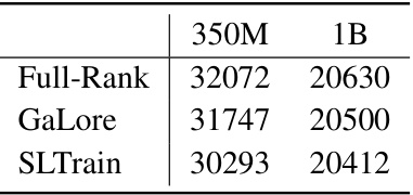
🔼 This table shows the throughput, measured in tokens per second, achieved by three different training methods (Full-Rank, GaLore, and SLTrain) on two different sizes of the LLaMA language model (350M and 1B parameters). The results highlight the relative efficiency of each method in terms of processing speed during training.
read the caption
Table 3: Throughput tokens/seconds for LLaMA 350M (on 1×80G A100 GPU) 1B (on 4×80G A100 GPUs).

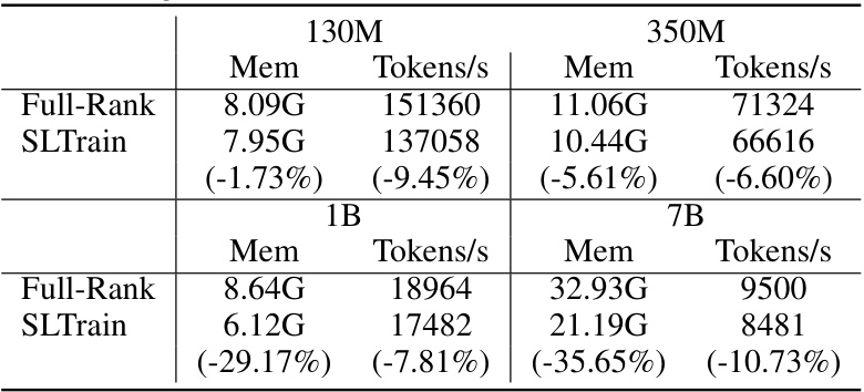
🔼 This table compares the performance of 8-bit GaLore and 8-bit SLTrain on the LLaMA 7B model, focusing on validation perplexity, actual memory footprint per GPU, and throughput (tokens per second). It highlights the memory efficiency gains achieved by SLTrain while maintaining a comparable level of performance.
read the caption
Table 4: Validation perplexity, actual memory footprint per GPU, and throughput tokens/seconds (Tokens/sec) for LLaMA 7B on 1.4B tokens.
🔼 This table compares the performance of different models in terms of perplexity, the number of parameters, and memory usage. It presents results for several LLAMA models of different sizes (60M, 130M, 350M, 1B parameters) pretrained using different methods: Full-Rank, Low-Rank, ReLORA, GaLore, and SLTrain. The SLTrain results use a fixed sparsity parameter (δ = 0.03). The table shows that SLTrain achieves comparable perplexity to Full-Rank while significantly reducing parameter count and memory requirements.
read the caption
Table 2: Validation perplexity (PPL(↓)), number of parameters in millions (Param), and estimated total memory cost in G (Mem). The perplexity results for all the baselines are taken from [59]. For SLTrain, we use the same rank as other baselines and fix δ = 0.03.
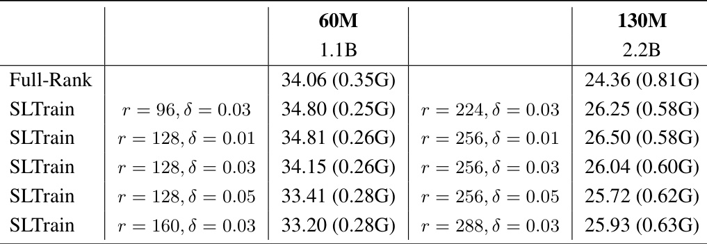
🔼 This table presents an ablation study comparing the performance of different parameterizations for the SLTrain model. It shows how changes in rank (r) and sparsity (δ) affect the validation perplexity (a lower score is better). The memory cost is also shown in gigabytes (G). This allows a comparison of model size against the performance improvement. Notably, the table displays results for various configurations of the SLTrain model alongside the full-rank baseline. It demonstrates that while adding more parameters generally improves performance, it is accompanied by an increase in memory.
read the caption
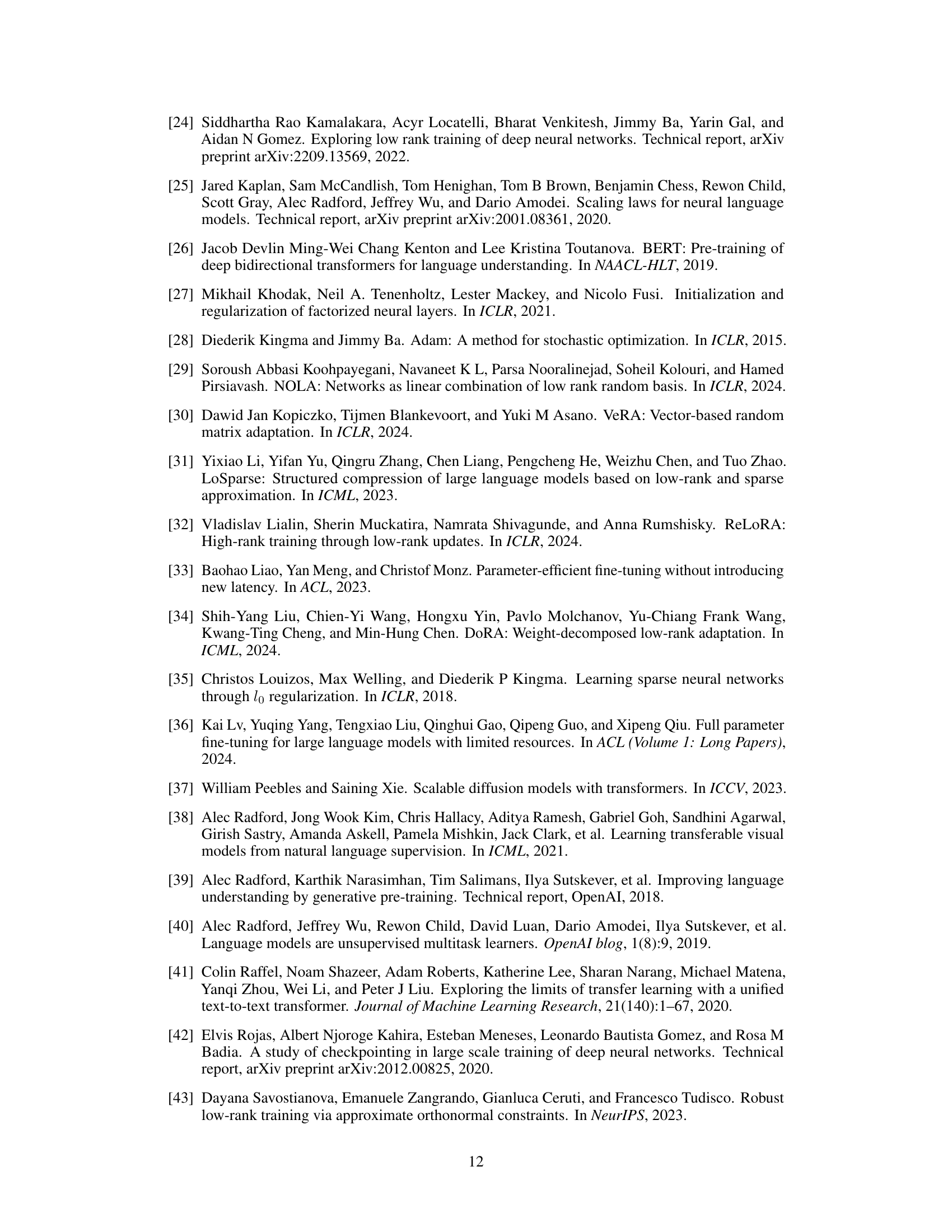
Table 6: Ablation comparison with low-rank and sparse parameterization along with change of rank r and sparsity δ. Validation perplexity (↓) and parameter size and estimated memory cost in brackets.

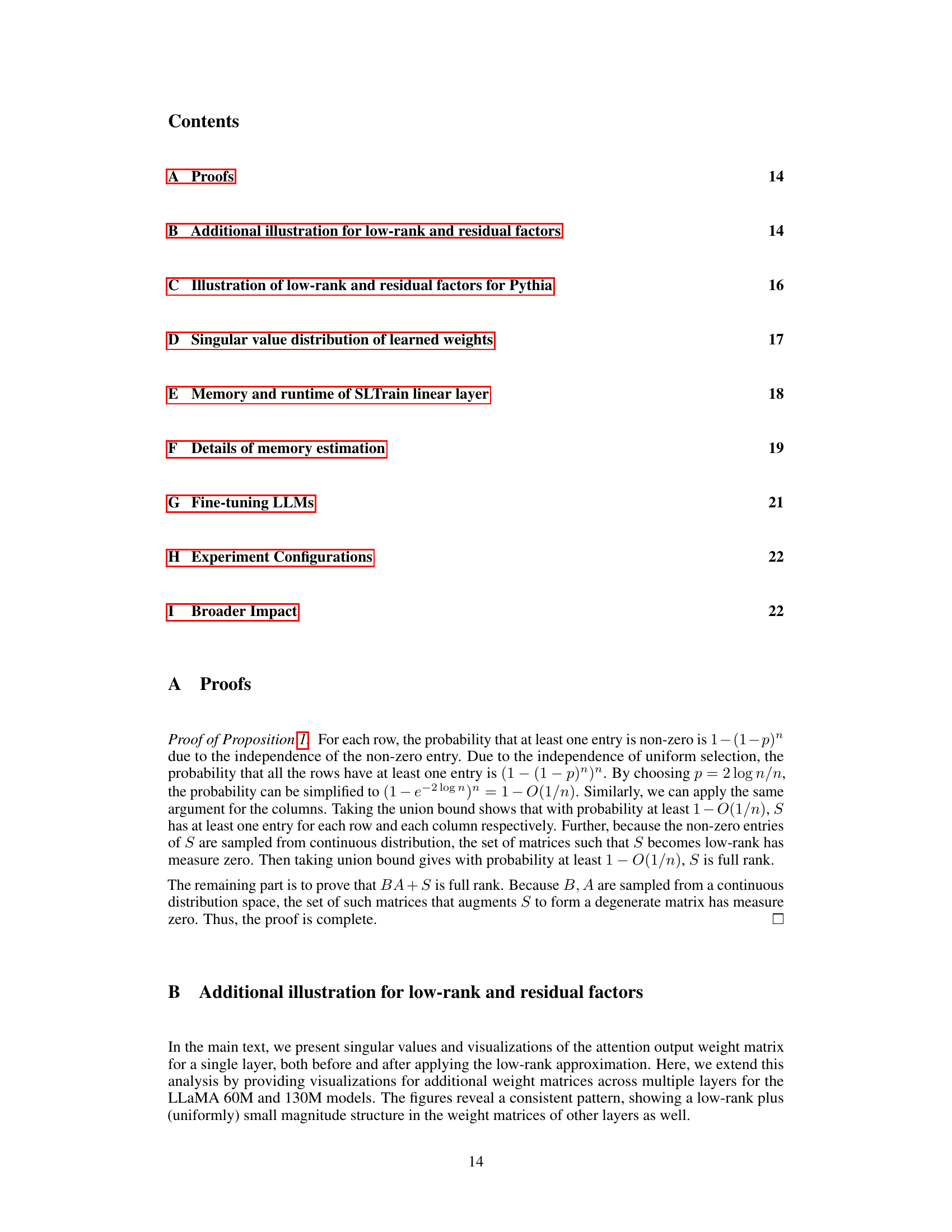
🔼 This table compares the performance of full-rank training and SLTrain with different sparsity ratios (δ) on LLaMA 350M and 1B models. It shows the validation perplexity, the number of parameters (in millions), and the maximum memory used per GPU. The results demonstrate that increasing the sparsity ratio while maintaining comparable perplexity leads to significant reductions in parameter size and memory usage.
read the caption
Table 7: Results training LLaMA 350M (with batch size=128 per GPU) and LLaMA 1B (with batch size=32 per GPU). Validation perplexity (PPL) (↓), number of parameters in millions (Param) and actual max memory allocated per GPU in G (Mem).

🔼 This table compares the performance of different models on the LLaMA dataset. The models are compared across three metrics: validation perplexity (PPL), number of parameters (in millions), and estimated memory cost (in gigabytes). The baselines used are full-rank training, low-rank training, ReLoRA, and GaLore. SLTrain results are shown, using the same rank as other methods, with δ fixed at 0.03. Lower PPL values are better, indicating higher model accuracy. Lower parameter and memory costs indicate more efficient models. The table helps to assess the trade-off between model performance and resource utilization.
read the caption
Table 2: Validation perplexity (PPL(↓)), number of parameters in millions (Param), and estimated total memory cost in G (Mem). The perplexity results for all the baselines are taken from [59]. For SLTrain, we use the same rank as other baselines and fix δ = 0.03.

🔼 This table presents the results of an ablation study on the impact of varying the rank (r) and sparsity (δ) parameters on the performance of the proposed SLTrain model. It compares the validation perplexity, parameter size, and estimated memory cost for different combinations of r and δ values, alongside a full-rank baseline. The results help in understanding the trade-off between model complexity and performance achieved by adjusting the hyperparameters.
read the caption
Table 6: Ablation comparison with low-rank and sparse parameterization along with change of rank r and sparsity δ. Validation perplexity (↓) and parameter size and estimated memory cost in brackets.

🔼 This table presents an ablation study comparing the performance of different configurations of the SLTrain model by varying the rank (r) and sparsity (δ) parameters. The results show the validation perplexity, parameter size (in millions), and estimated memory cost (in gigabytes) for different combinations of r and δ. The goal is to evaluate how the balance of low-rank and sparse components affect model performance and resource usage.
read the caption
Table 6: Ablation comparison with low-rank and sparse parameterization along with change of rank r and sparsity δ. Validation perplexity (↓) and parameter size and estimated memory cost in brackets.

🔼 This table shows the hyperparameters used for fine-tuning the RoBERTa base model with SLTrain on the GLUE benchmark. It specifies the batch size, number of epochs, rank (r), learning rate, sparsity (δ), and scaling factor (α) for each of the eight GLUE tasks (COLA, STS-B, MRPC, RTE, SST-2, MNLI, QNLI, QQP). The rank and epochs are consistent with the settings in the paper referenced by [59], while the other hyperparameters are tuned specifically for SLTrain on this fine-tuning task.
read the caption
Table 11: Hyperparameters of SLTrain for fine-tuning. The batch size, number of epochs and rank r follows from the choice in [59].

🔼 This table compares the performance of different model training methods on various sizes of the LLaMA language model. The metrics compared are validation perplexity (PPL), number of parameters (in millions), and estimated total memory cost (in gigabytes). The results show SLTrain’s comparable performance to full-rank training with reduced parameter size and memory cost. The baseline methods for comparison include Full-Rank, Low-Rank, ReLORA, and GaLore. For SLTrain, a consistent sparsity ratio (δ) of 0.03 is used across different model sizes.
read the caption
Table 2: Validation perplexity (PPL(↓)), number of parameters in millions (Param), and estimated total memory cost in G (Mem). The perplexity results for all the baselines are taken from [59]. For SLTrain, we use the same rank as other baselines and fix δ = 0.03.
Full paper#
