TL;DR#
Deep learning models are computationally expensive, especially on mobile and embedded devices with limited resources. Depthwise Separable Convolutions (DSC) are widely used to reduce model size and computation, but pruning DSC models effectively remains challenging due to the already compact nature of DSC. Existing pruning techniques often struggle to maintain accuracy while achieving significant speedups on GPUs.
DEPrune tackles these challenges by introducing a novel pruning method tailored for DSC on GPUs. It uses a fine-grained pruning approach coupled with techniques like balanced workload tuning (BWT) and hardware-aware sparsity recalibration (HSR) to maximize GPU parallelism and maintain accuracy. Experimental results show that DEPrune achieves substantial speedups (up to 3.74x) on various models like EfficientNet-B0 without sacrificing accuracy, demonstrating its potential for efficient AI deployment on resource-constrained devices.
Key Takeaways#
Why does it matter?#
This paper is important because it presents a novel pruning method, DEPrune, that significantly accelerates deep learning models on GPUs by focusing on depthwise separable convolutions. This addresses a critical challenge in deploying large models on resource-constrained devices. The techniques introduced, particularly balanced workload tuning and hardware-aware sparsity recalibration, offer valuable insights for optimizing GPU utilization and achieving further speed improvements in pruned networks. The findings directly contribute to the ongoing research on efficient deep learning, and open avenues for future work in hardware-aware model optimization and resource-efficient AI.
Visual Insights#
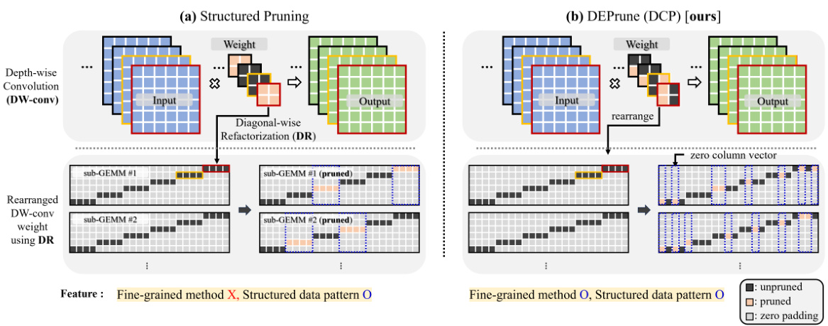
🔼 This figure compares structured pruning and DEPrune (DCP) methods. It illustrates how depthwise convolution is restructured into multiple sub-GEMMs (general matrix-matrix multiplications) using diagonal-wise refactorization (DR) for better GPU parallelism. The figure highlights that while both methods achieve structured sparsity, DEPrune is more fine-grained, leading to more efficient pruning and better performance.
read the caption
Figure 1: Depth-wise convolution is rearranged to multi sub-GEMM on GPU by applying Diagonal-wise Refactorization (DR). The ‘X’ and ‘O’ symbols indicate the absence and presence of corresponding characteristics for each method. Applying (a) Structured Pruning and (b) DEPrune (DCP) to multi sub-GEMM results in a structured data pattern. But (b) DEPrune (DCP) is more fine-grained method than (a) Structured Pruning.
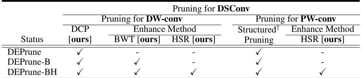
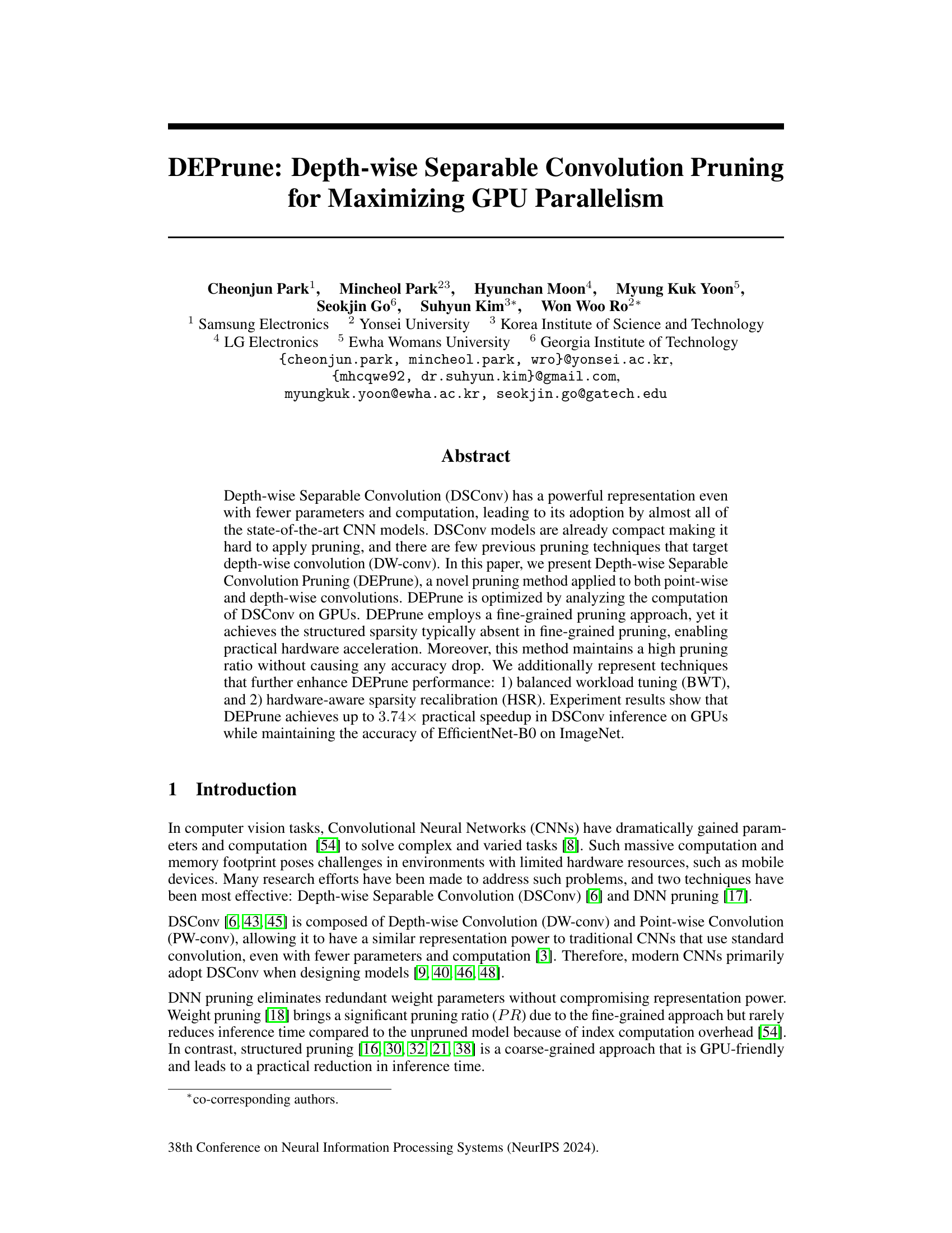
🔼 This table summarizes the terminology used in the paper to describe the different variations of the DEPrune method. It shows the status (applied or not) of the core Depth-wise Convolution Pruning (DCP) method, along with optional enhancements: Balanced Workload Tuning (BWT) and Hardware-aware Sparsity Recalibration (HSR), applied separately to DW-conv and PW-conv layers. It clarifies which pruning methods are used for depthwise and pointwise convolutions in each variant of DEPrune.
read the caption
Table 1: Terminology of DEPrune method. This symbol (†) means ‘we apply our methodology to determine which PW-conv to prune for better performance (Sec. 4.2)’. BWT and HSR are our proposed method to enhance DEPrune. BWT and HSR are described in Sec. 5.1 and Sec. 5.2, respectively. This symbol (√) means ‘Applied’.
In-depth insights#
GPU Parallelism#
The research paper explores optimizing GPU parallelism for depth-wise separable convolutions (DSC). Depth-wise separable convolutions, while computationally efficient, don’t always fully utilize GPU resources due to their structure. The core idea is to enhance GPU utilization by strategically pruning the convolutional weights. The authors present a novel pruning method called DEPrune, which carefully analyzes the computation of DSC on GPUs for fine-grained pruning while maintaining a structured sparsity, crucial for hardware acceleration. DEPrune’s effectiveness stems from its fine-grained approach, which avoids the significant accuracy loss associated with coarser methods while still achieving the structured sparsity needed for practical hardware acceleration. Furthermore, the paper introduces techniques like balanced workload tuning (BWT) to handle workload imbalances among different processing units on the GPU, thereby maximizing parallel efficiency. Hardware-aware sparsity recalibration (HSR) further refines the pruning process by aligning it with the GPU’s execution units, improving speed further. The combination of DEPrune, BWT, and HSR leads to substantial speedups in inference time on GPUs while maintaining accuracy. This highlights the importance of considering hardware specifics (like GPU architecture and tile size) when developing efficient pruning strategies for deep learning models.
DSConv Pruning#
DSConv pruning techniques aim to improve the efficiency of depthwise separable convolutions (DSCONV) by removing less important parameters. The core challenge lies in the inherent compactness of DSConv, making it difficult to prune without significant accuracy loss. Existing pruning methods often struggle to effectively target depthwise convolutions, leading to suboptimal results. A promising approach involves analyzing the computational characteristics of DSConv on GPUs to identify and remove redundant weights in a structured manner, maintaining a high pruning ratio while minimizing accuracy degradation. This requires careful consideration of the GPU architecture and parallel processing capabilities to ensure the pruned model leverages hardware acceleration effectively. Furthermore, techniques like balanced workload tuning and hardware-aware sparsity recalibration are crucial to overcome issues such as workload imbalance between processing units and unaligned pruning, thereby maximizing the speedup achievable through pruning.
DEPrune Method#
The DEPrune method, a novel pruning technique for depthwise separable convolutions (DSC), focuses on optimizing GPU parallelism. It’s a fine-grained approach, unlike traditional structured pruning methods, yet it cleverly achieves structured sparsity by leveraging diagonal-wise refactorization (DR). DR transforms the depthwise convolution into multiple GEMMs, facilitating efficient GPU parallelization. By performing fine-grained pruning within these rearranged GEMMs, DEPrune can achieve high pruning ratios without significant accuracy loss. Furthermore, DEPrune’s optimizations extend beyond the initial pruning, including balanced workload tuning (BWT) to mitigate the performance penalty of uneven pruning across different sub-GEMMs and hardware-aware sparsity recalibration (HSR) to optimize GPU utilization and reduce memory access overhead. The combination of these techniques makes DEPrune a potent method for accelerating DSConv-based models while preserving accuracy.
Workload Tuning#
Workload tuning, in the context of optimizing depth-wise separable convolutions (DSConv) for GPU parallelism, addresses the imbalance in computational workload across different processing units. This imbalance arises because the pruning ratios applied to various sub-GEMMs (General Matrix-Matrix Multiplications) within the DSConv operation may vary, leading to some processing units waiting idly for others to finish. Balanced Workload Tuning (BWT) aims to mitigate this by strategically setting similar target pruning ratios for each sub-GEMM. This ensures more uniform resource utilization, ultimately improving GPU efficiency and reducing inference time. The effectiveness of BWT depends on the interplay between the fine-grained pruning approach and the granularities of GPU parallelization. Thus, a careful consideration of these aspects is crucial in successfully implementing BWT to achieve significant speedup without sacrificing accuracy. Hardware-aware Sparsity Recalibration (HSR) further refines BWT’s performance by aligning pruning with GPU’s execution units, resolving potential memory access inefficiencies. The interplay between BWT and HSR creates a robust and efficient approach to maximize GPU performance.
Sparsity Limits#
The concept of ‘sparsity limits’ in the context of a research paper likely refers to the inherent boundaries in achieving extreme sparsity in neural networks while maintaining acceptable performance. Pushing sparsity too far can lead to significant accuracy degradation, as crucial information is inadvertently pruned. The research likely explores techniques to overcome these limits, potentially examining architectural modifications, advanced pruning algorithms (e.g., structured pruning, dynamic sparsity), or retraining strategies that account for the removal of connections. Understanding these limits is crucial for developing efficient and practical sparse models, striking a balance between reduced computational cost and the preservation of accuracy. The paper might investigate different types of sparsity (e.g., weight sparsity, filter sparsity, channel sparsity), examining if some sparsity patterns are more robust than others. Determining and characterizing these limits for various network architectures and datasets is a key contribution, offering valuable guidelines for future research in neural network compression.
More visual insights#
More on figures
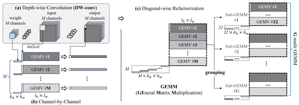
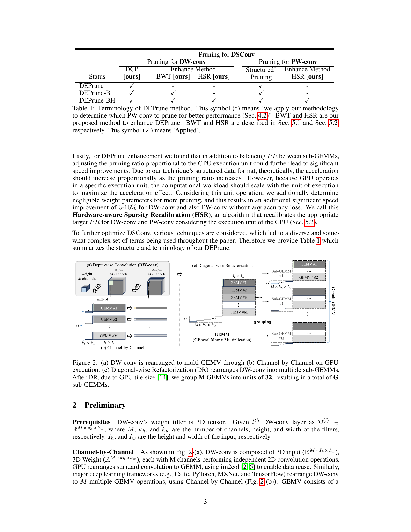
🔼 This figure illustrates the transformation of depthwise convolution (DW-conv) operations on a GPU. It starts with a standard channel-by-channel approach (b), where DW-conv is broken down into multiple GEMV (General Matrix-Vector Multiplication) operations. The key improvement is shown in (c), where Diagonal-wise Refactorization (DR) restructures the DW-conv weights and inputs into multiple smaller sub-GEMMs (General Matrix-Matrix Multiplication), significantly improving GPU parallelism. The grouping of GEMVs into units of 32 is explained due to the GPU’s tile size limitation, resulting in a total of ‘G’ sub-GEMMs. The figure visually represents how the process optimizes GPU utilization.
read the caption
Figure 2: (a) DW-conv is rearranged to multi GEMV through (b) Channel-by-Channel on GPU execution. (c) Diagonal-wise Refactorization (DR) rearranges DW-conv into multiple sub-GEMMs. After DR, due to GPU tile size [14], we group M GEMVs into units of 32, resulting in a total of G sub-GEMMs.
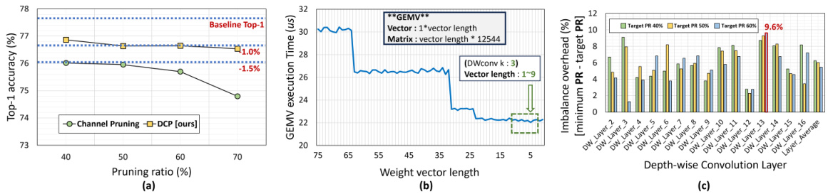
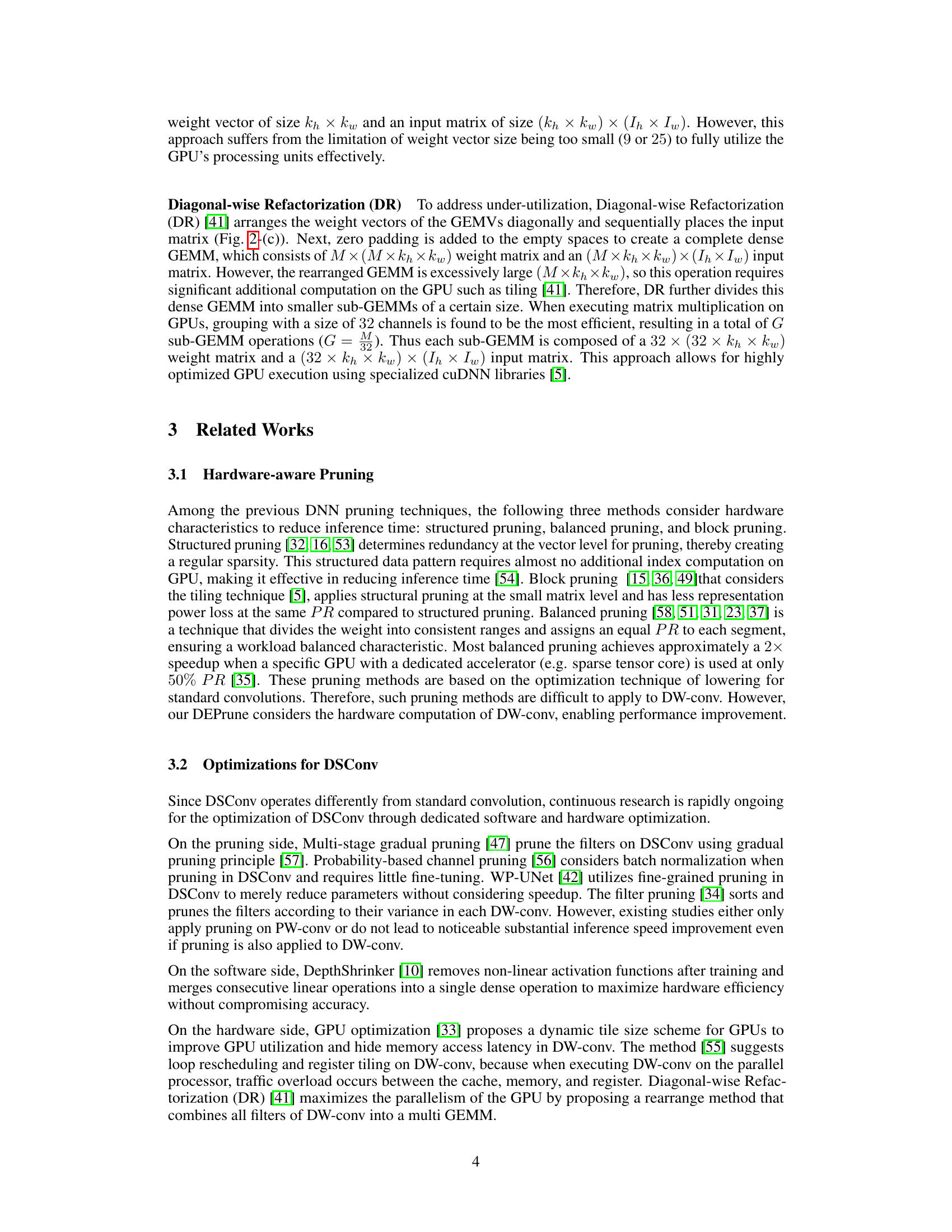
🔼 This figure compares the accuracy drop of channel pruning and DCP methods on EfficientNet-B0 using ImageNet, showing that DCP has a lower accuracy drop at the same pruning ratio. It also shows the GEMV execution time and imbalance overhead of Mobilenet-V2 on ImageNet, illustrating the efficiency gain of DCP and the workload imbalance problem.
read the caption
Figure 3: (a) Comparison of accuracy drop between DCP and channel pruning on EfficientNet-B0 using ImageNet. (b) Measurement of the GEMV execution time of DW-conv 6th layer of EfficientNet-B0 on GPU. (c) Measurement of imbalance overhead of Mobilenet-V2 on ImageNet. The imbalance overhead is the difference between minimum sub-GEMM pruning ratio (PR) and layer's target PR.
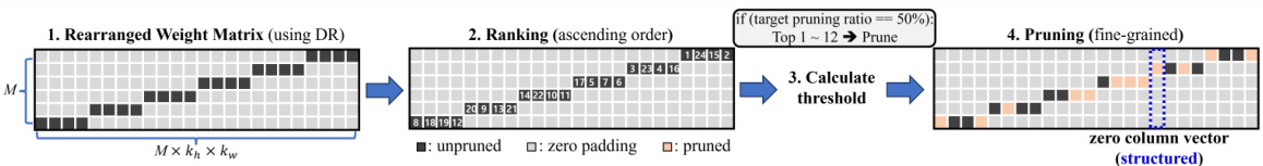
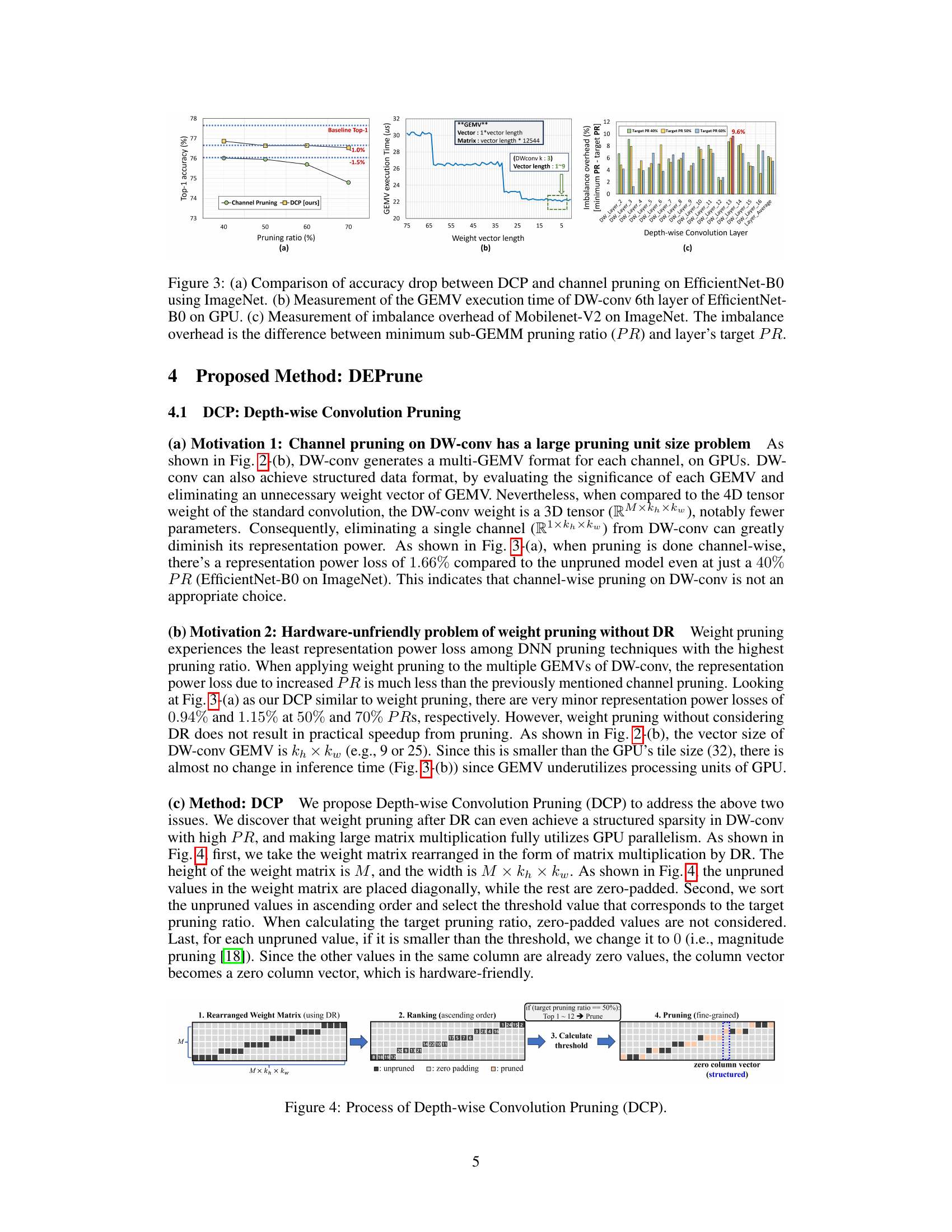
🔼 This figure illustrates the four steps involved in Depth-wise Convolution Pruning (DCP). First, the weight matrix is rearranged using Diagonal-wise Refactorization (DR), resulting in a diagonal pattern of non-zero weights. Second, these non-zero weights are ranked in ascending order. Third, a threshold value is calculated based on the target pruning ratio. Finally, fine-grained pruning is applied, setting any weight below the threshold to zero, resulting in a structured sparsity pattern where entire columns become zero vectors.
read the caption
Figure 4: Process of Depth-wise Convolution Pruning (DCP).
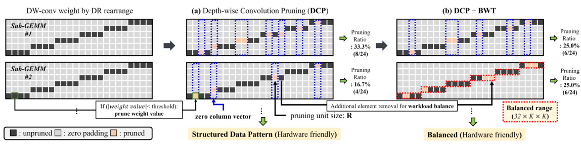
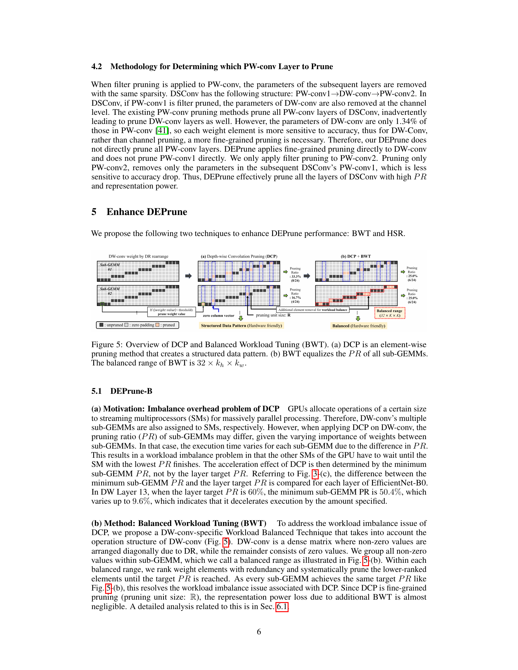
🔼 This figure illustrates the Depth-wise Convolution Pruning (DCP) method and how Balanced Workload Tuning (BWT) improves it. DCP performs fine-grained pruning on depth-wise convolutions rearranged using Diagonal-wise Refactorization (DR), resulting in a structured, hardware-friendly sparsity pattern. However, DCP can lead to workload imbalance across processing units due to varying pruning ratios in different sub-GEMMs. BWT addresses this by ensuring equal pruning ratios across all sub-GEMMs, improving GPU utilization and performance. The figure visually compares the pruning process and resulting sparsity patterns for both DCP and DCP+BWT.
read the caption
Figure 5: Overview of DCP and Balanced Workload Tuning (BWT). (a) DCP is an element-wise pruning method that creates a structured data pattern. (b) BWT equalizes the PR of all sub-GEMMs. The balanced range of BWT is 32 × kh × kw.
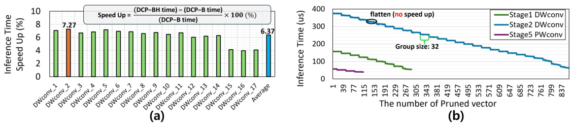
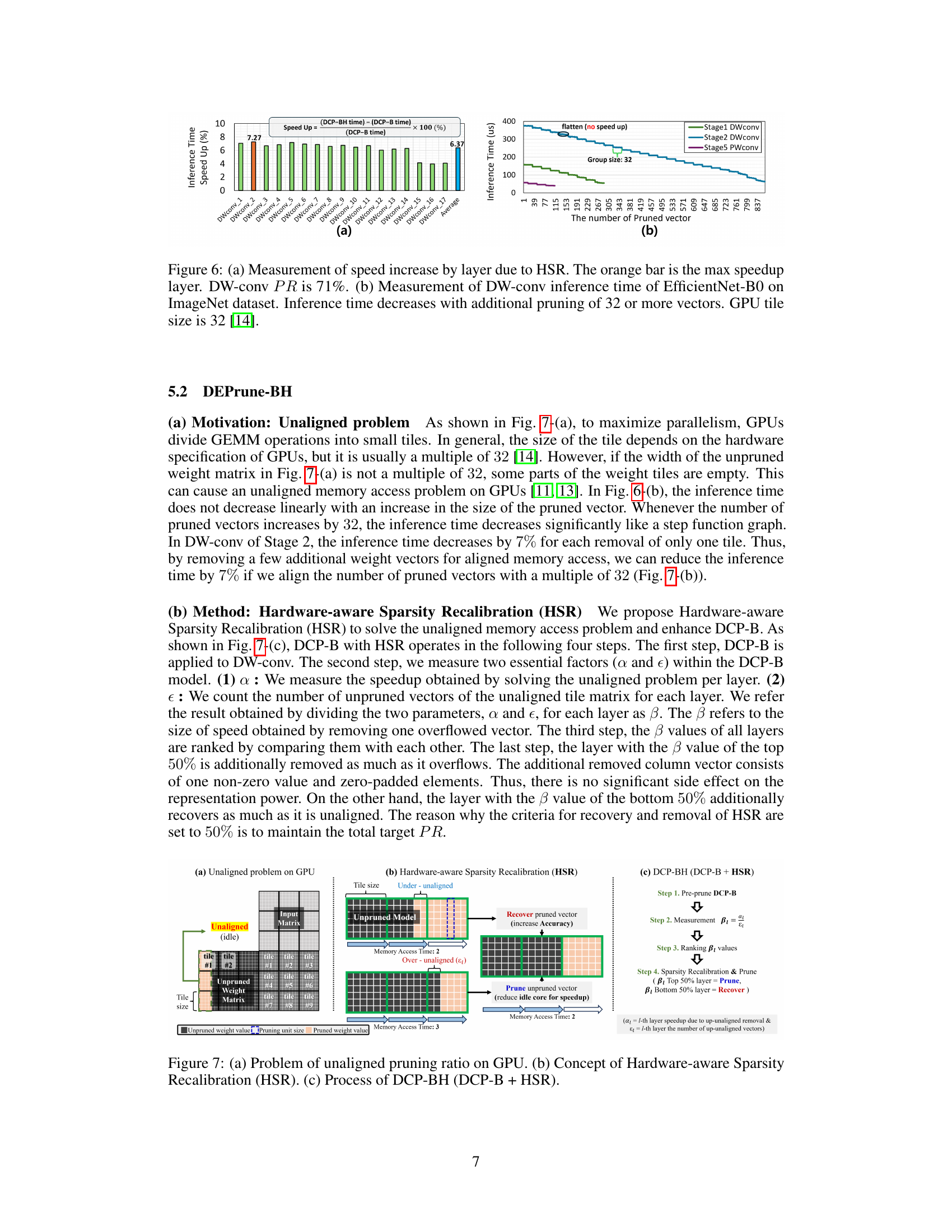
🔼 Figure 6 shows two graphs. Graph (a) displays the speedup percentage for each layer of DW-conv after applying HSR, showing a maximum speedup of 7.27%. Graph (b) illustrates the effect of pruning on DW-conv inference time, demonstrating that inference time significantly decreases when 32 or more vectors are pruned.
read the caption
Figure 6: (a) Measurement of speed increase by layer due to HSR. The orange bar is the max speedup layer. DW-conv PR is 71%. (b) Measurement of DW-conv inference time of EfficientNet-B0 on ImageNet dataset. Inference time decreases with additional pruning of 32 or more vectors. GPU tile size is 32 [14].
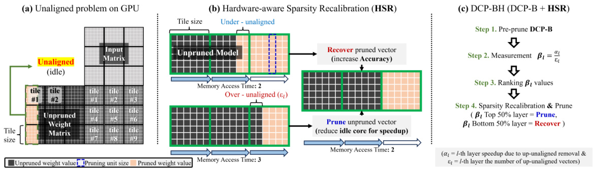
🔼 This figure illustrates the problem of unaligned pruning on GPUs, which leads to inefficiency. It introduces Hardware-aware Sparsity Recalibration (HSR) as a solution. Part (a) shows how unaligned pruning results in idle processing units. Part (b) details HSR, which adjusts pruning to align with GPU tile sizes to maximize efficiency. Part (c) outlines the steps of DCP-BH (DCP-B + HSR), combining DCP-B with HSR for optimal performance.
read the caption
Figure 7: (a) Problem of unaligned pruning ratio on GPU. (b) Concept of Hardware-aware Sparsity Recalibration (HSR). (c) Process of DCP-BH (DCP-B + HSR).
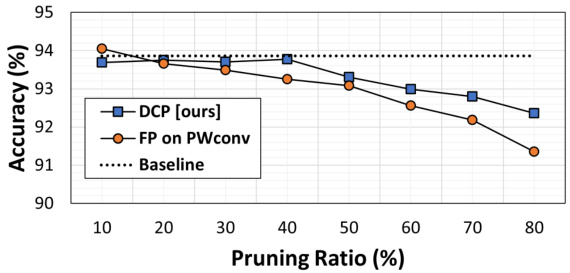
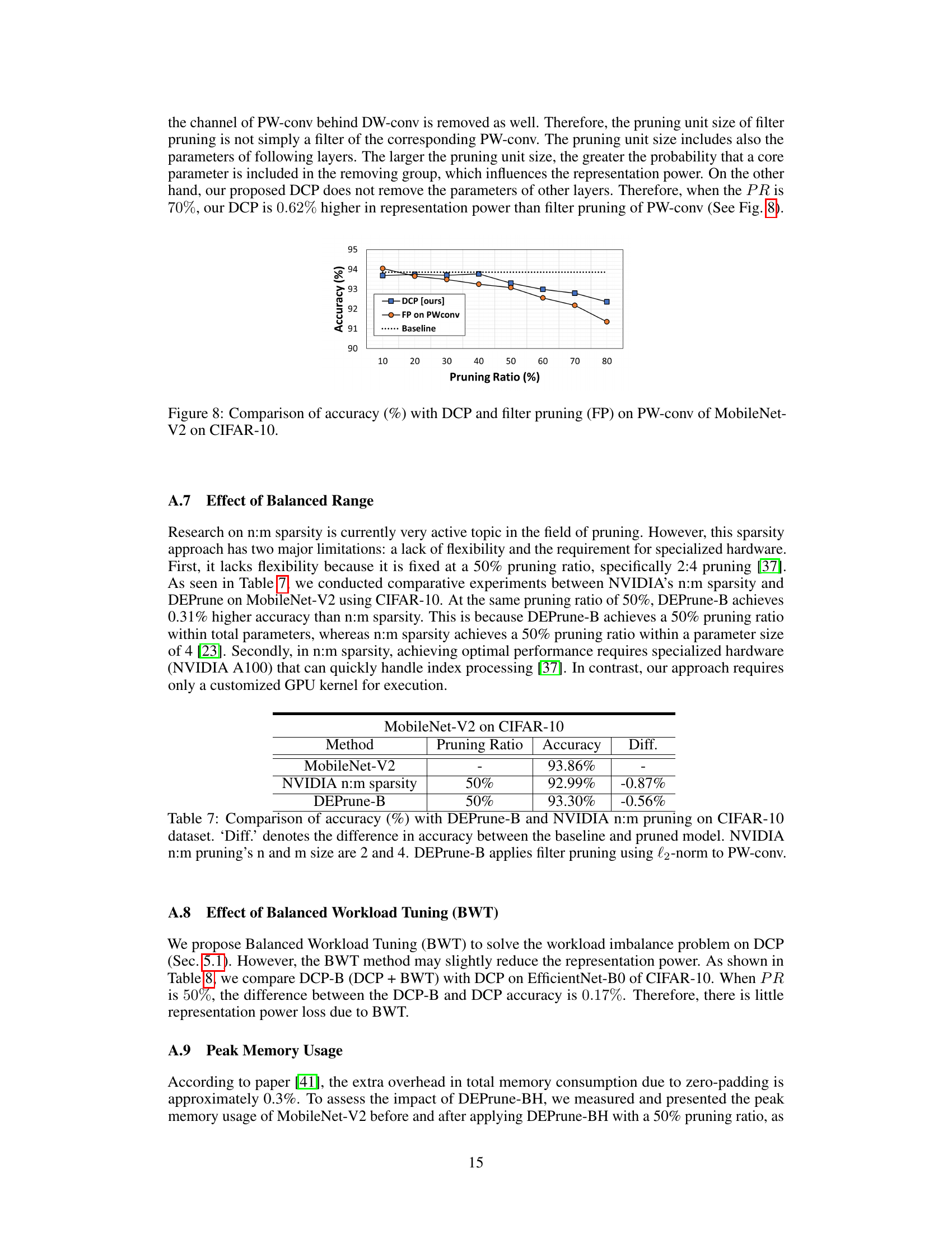
🔼 The figure shows a comparison of accuracy between DCP (Depthwise Convolution Pruning) and filter pruning on the PW-conv (Pointwise Convolution) layers of the MobileNet-V2 model, trained on the CIFAR-10 dataset. The x-axis represents the pruning ratio (percentage of weights removed), and the y-axis represents the top-1 accuracy. The graph shows that DCP maintains higher accuracy than filter pruning across various pruning ratios. A horizontal dotted line represents the baseline accuracy without pruning.
read the caption
Figure 8: Comparison of accuracy (%) with DCP and filter pruning (FP) on PW-conv of MobileNet-V2 on CIFAR-10.
More on tables
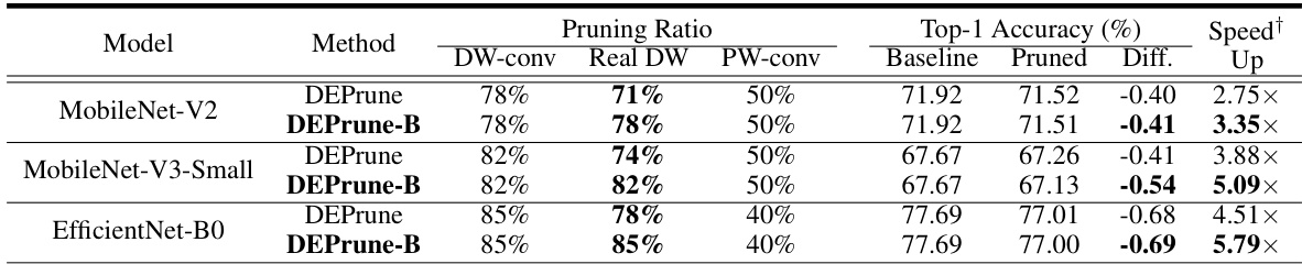
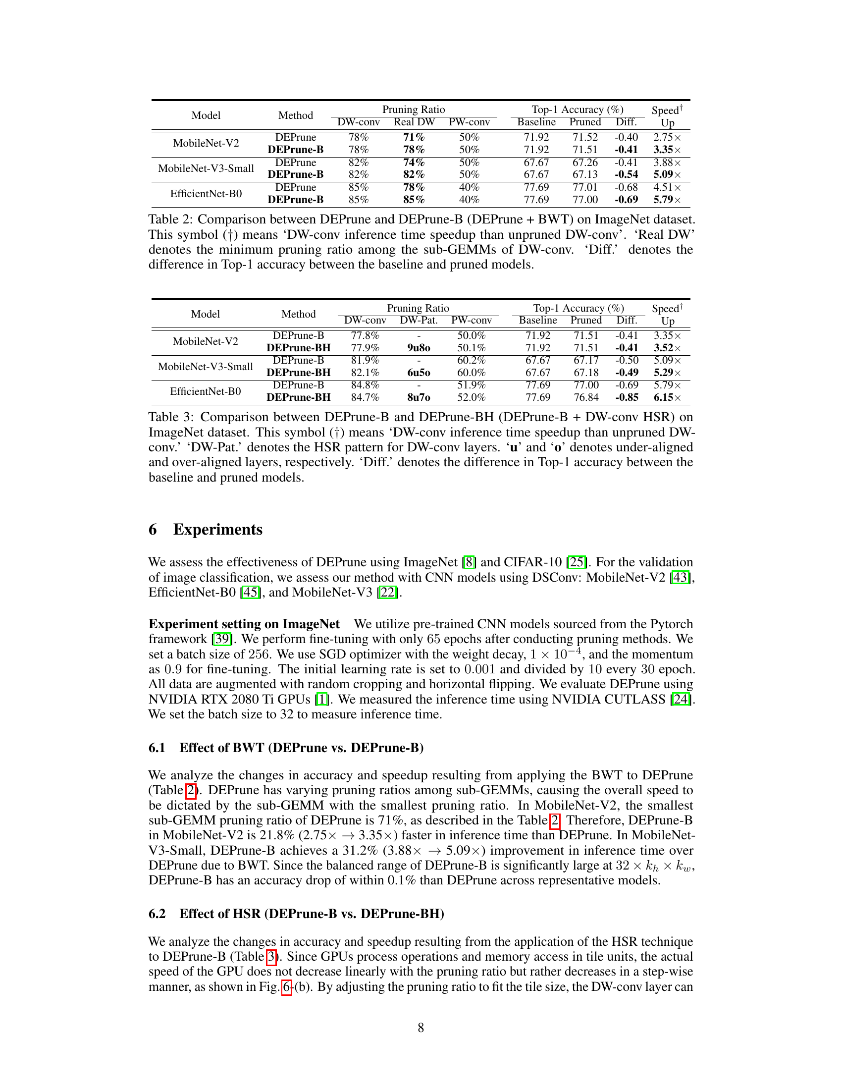
🔼 This table compares the performance of DEPrune and DEPrune-B (which incorporates Balanced Workload Tuning) on the ImageNet dataset using three different CNN models. It shows the pruning ratios achieved for depthwise convolutions (DW-conv), the actual minimum pruning ratio among the sub-GEMMs of DW-conv, the pruning ratio for pointwise convolutions (PW-conv), the baseline top-1 accuracy, the top-1 accuracy after pruning, the difference in accuracy, and the speedup achieved. The speedup is relative to the unpruned DW-conv.
read the caption
Table 2: Comparison between DEPrune and DEPrune-B (DEPrune + BWT) on ImageNet dataset. This symbol (†) means ‘DW-conv inference time speedup than unpruned DW-conv’. ‘Real DW’ denotes the minimum pruning ratio among the sub-GEMMs of DW-conv. ‘Diff.’ denotes the difference in Top-1 accuracy between the baseline and pruned models.
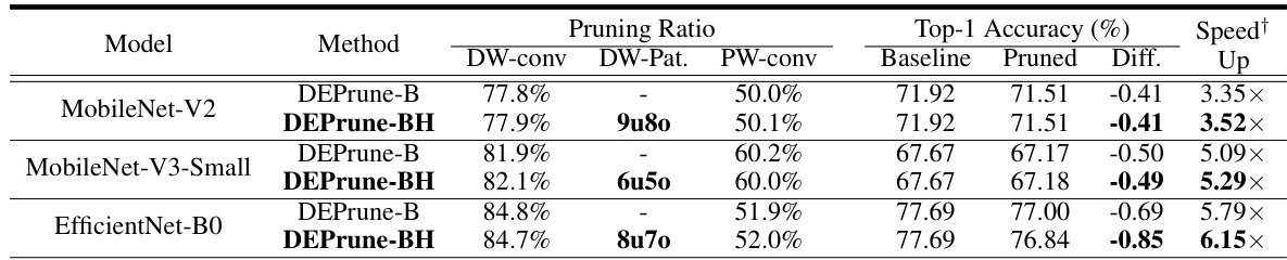
🔼 This table compares the performance of DEPrune-B and DEPrune-BH (which incorporates Hardware-aware Sparsity Recalibration or HSR) on the ImageNet dataset. It shows the pruning ratios achieved for depthwise convolution (DW-conv) and pointwise convolution (PW-conv), along with the resulting top-1 accuracy and speedup. The ‘DW-Pat’ column indicates the pattern of HSR applied to DW-conv layers, classifying them as under-aligned (u) or over-aligned (o). The ‘Diff’ column highlights the difference in top-1 accuracy between the pruned and baseline models.
read the caption
Table 3: Comparison between DEPrune-B and DEPrune-BH (DEPrune-B + DW-conv HSR) on ImageNet dataset. This symbol (†) means ‘DW-conv inference time speedup than unpruned DW-conv.’ ‘DW-Pat.’ denotes the HSR pattern for DW-conv layers. ‘u’ and ‘o’ denotes under-aligned and over-aligned layers, respectively. ‘Diff.’ denotes the difference in Top-1 accuracy between the baseline and pruned models.
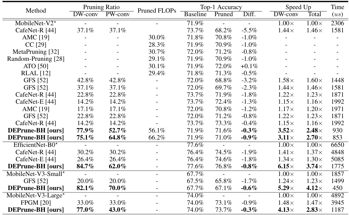
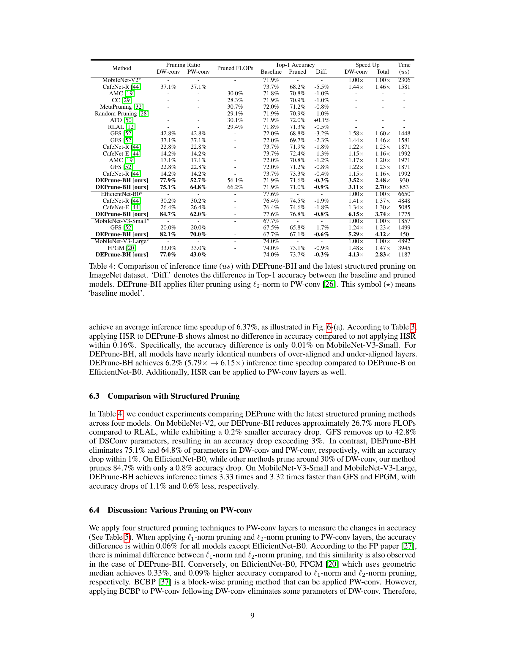
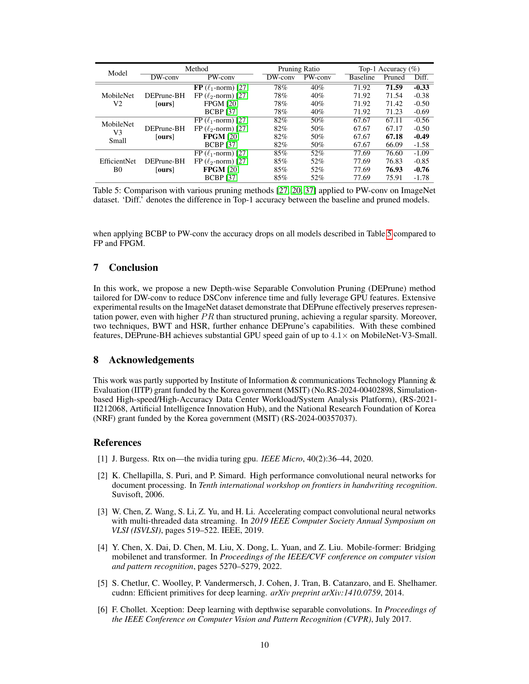
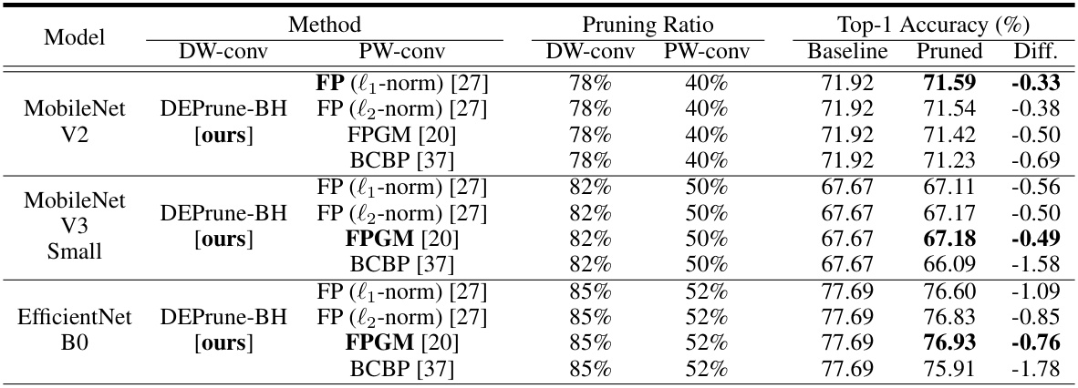
🔼 This table compares the inference time and top-1 accuracy of DEPrune-BH against other state-of-the-art structured pruning methods on the ImageNet dataset using three different CNN models (MobileNet-V2, MobileNet-V3-Small, EfficientNet-B0). It shows the pruning ratios applied to depthwise and pointwise convolutions, the resulting pruned FLOPs, the difference in top-1 accuracy compared to the baseline, and the speedup achieved by DEPrune-BH in both depthwise and total inference time. The baseline models are unpruned versions.
read the caption
Table 4: Comparison of inference time (µs) with DEPrune-BH and the latest structured pruning on ImageNet dataset. ‘Diff.’ denotes the difference in Top-1 accuracy between the baseline and pruned models. DEPrune-BH applies filter pruning using l2-norm to PW-conv. This symbol (*) means ‘baseline model.’
🔼 This table compares the performance of DEPrune-B and DEPrune-BH on the ImageNet dataset. DEPrune-BH adds Hardware-aware Sparsity Recalibration (HSR) to DEPrune-B. The table shows the pruning ratios for DW-conv and PW-conv layers, the Top-1 accuracy (comparing pruned models to the baseline), and the speedup achieved with DW-conv. It also indicates whether layers are under-aligned (u) or over-aligned (o) after HSR, highlighting the impact of this technique on performance and accuracy.
read the caption
Table 3: Comparison between DEPrune-B and DEPrune-BH (DEPrune-B + DW-conv HSR) on ImageNet dataset. This symbol (†) means ‘DW-conv inference time speedup than unpruned DW-conv.’ ‘DW-Pat.’ denotes the HSR pattern for DW-conv layers. ‘u’ and ‘o’ denotes under-aligned and over-aligned layers, respectively. ‘Diff.’ denotes the difference in Top-1 accuracy between the baseline and pruned models.
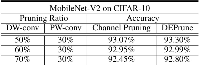
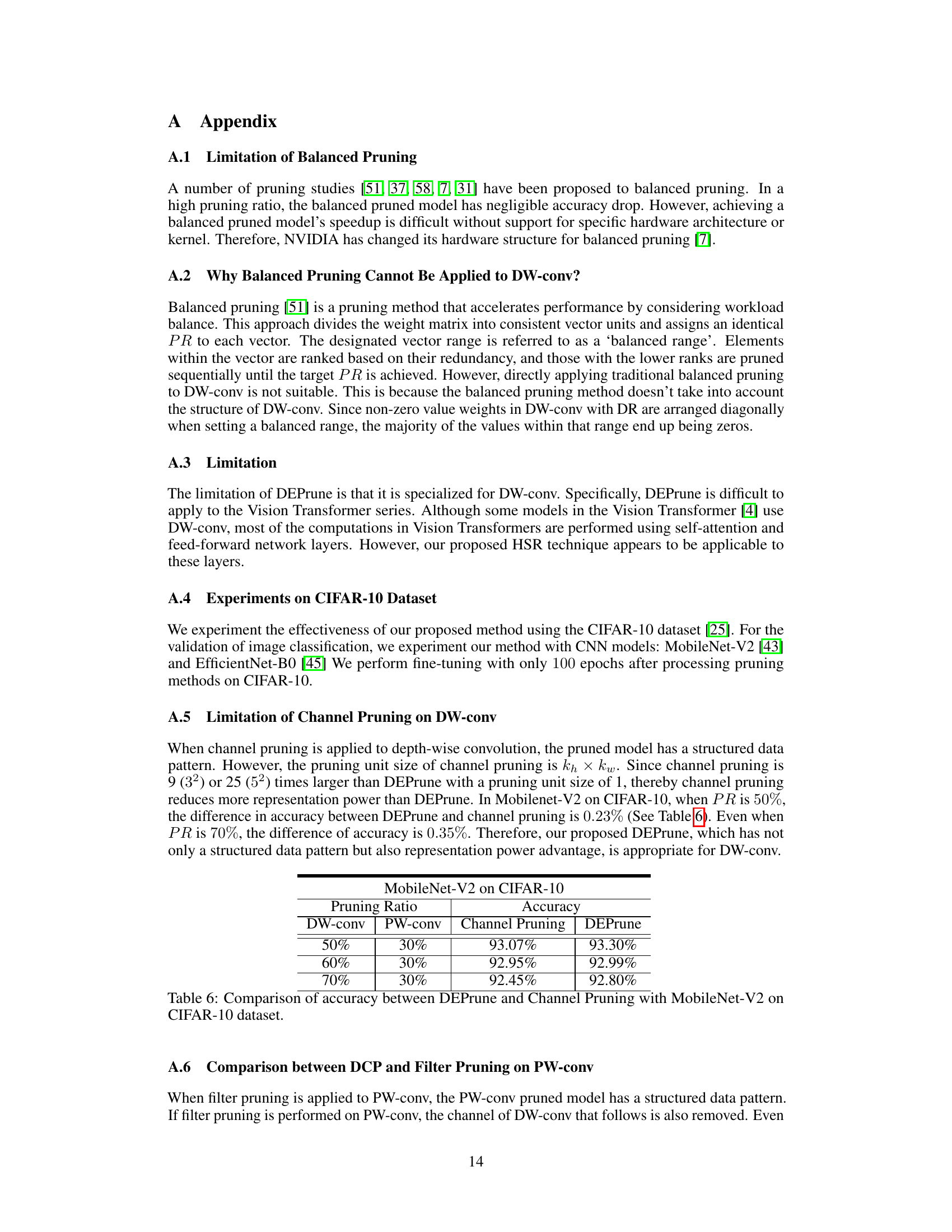
🔼 This table compares the accuracy of MobileNet-V2 on the CIFAR-10 dataset when using channel pruning and DEPrune at different pruning ratios for both depthwise and pointwise convolutional layers. It shows that DEPrune consistently achieves slightly higher accuracy than channel pruning, even at higher pruning ratios.
read the caption
Table 6: Comparison of accuracy between DEPrune and Channel Pruning with MobileNet-V2 on CIFAR-10 dataset.
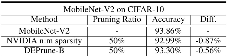
🔼 This table compares the accuracy of MobileNet-V2 on the CIFAR-10 dataset after applying three different pruning methods: no pruning (baseline), NVIDIA’s n:m sparsity pruning (50% pruning ratio), and the proposed DEPrune-B method (50% pruning ratio). It shows the accuracy drop (‘Diff.’) compared to the baseline for each pruning technique. Note that DEPrune-B uses a specific filter pruning technique (l2-norm) applied to the pointwise convolutions (PW-conv).
read the caption
Table 7: Comparison of accuracy (%) with DEPrune-B and NVIDIA n:m pruning on CIFAR-10 dataset. ‘Diff.’ denotes the difference in accuracy between the baseline and pruned model. NVIDIA n:m pruning’s n and m size are 2 and 4. DEPrune-B applies filter pruning using l2-norm to PW-conv.
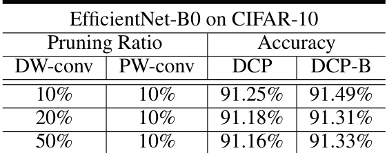
🔼 This table presents the results of applying Depthwise Convolution Pruning (DCP) and Balanced Workload Tuning (BWT) enhanced DCP (DCP-B) to the EfficientNet-B0 model on the CIFAR-10 dataset. It shows the accuracy achieved at different pruning ratios for both DW-conv and PW-conv layers. The comparison highlights the impact of BWT on the model’s accuracy.
read the caption
Table 8: Comparison between DCP and DCP-B of EfficientNet-B0 on CIFAR-10 dataset.
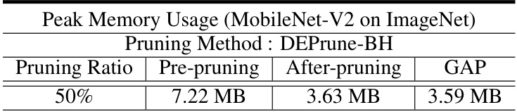
🔼 This table shows the peak memory usage (in MB) of MobileNet-V2 on the ImageNet dataset before and after applying the DEPrune-BH pruning method with a 50% pruning ratio. It highlights the memory reduction achieved by the method. The ‘GAP’ column shows the difference in peak memory usage between the pre-pruned and post-pruned model.
read the caption
Table 9: Analysis of Peak Memory Usage (MB) with DEPrune-BH on ImageNet dataset. ‘GAP’ means the after-pruning peak memory usage difference rate compared to pre-pruning. DEPrune-BH applies filter pruning using l2-norm to PW-conv.
Full paper#