TL;DR#
Many real-world applications heavily rely on time series data analysis for tasks like forecasting and anomaly detection. However, missing values are a common problem, significantly affecting the performance of existing methods. Current imputation methods primarily focus on data restoration, neglecting the impact on downstream tasks. This leads to suboptimal results as an imputation method that is excellent in general may not perform well in a specific task.
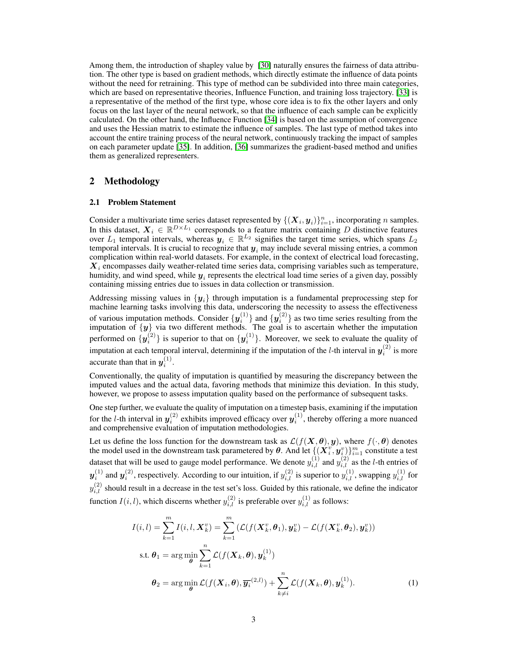
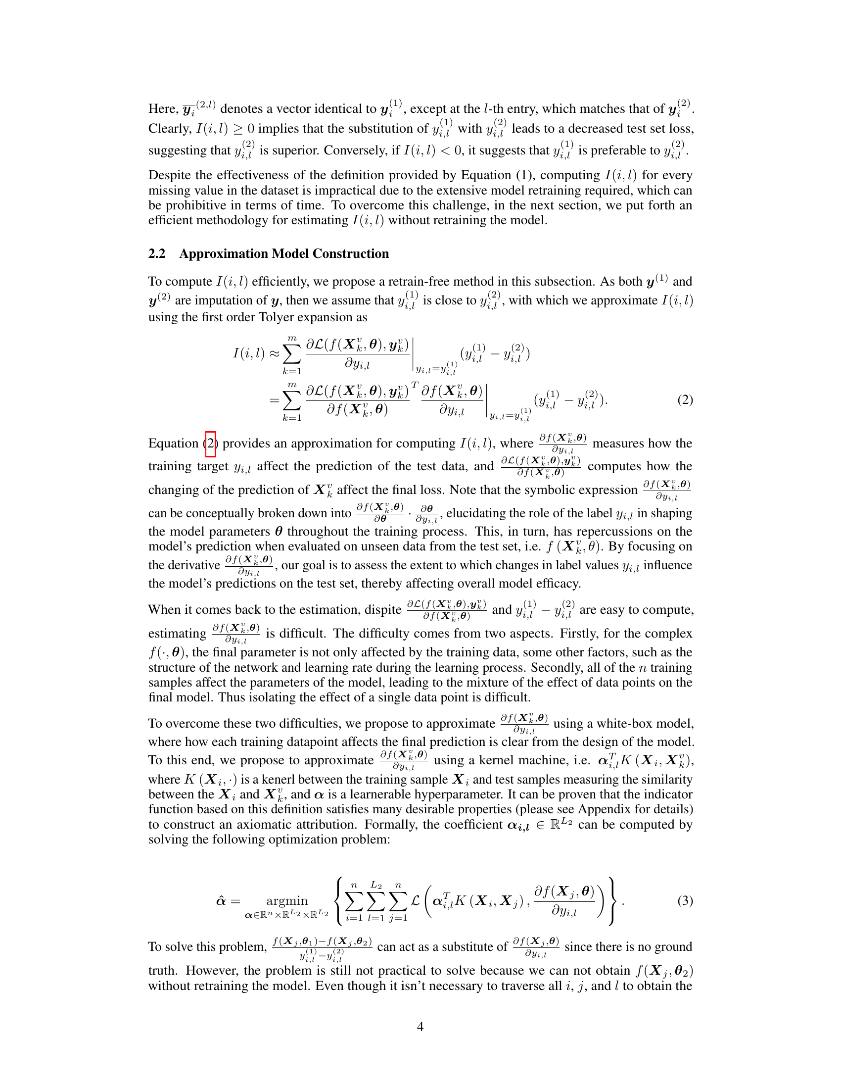
This paper tackles this issue by introducing a task-oriented evaluation strategy. It combines time series imputation with neural network models used for downstream tasks. This approach estimates the benefit of various imputation methods for specific downstream tasks without repeatedly retraining the model. The research also presents a similarity calculation method that speeds up the evaluation process and proposes a framework guided by maximizing the gains of downstream tasks, which leads to superior results. The key contributions include a novel task-oriented evaluation method, an efficient similarity calculation method, and a time series imputation framework guided by downstream task performance.
Key Takeaways#
Why does it matter?#
This paper is important because it addresses a critical challenge in time series analysis: handling missing data effectively for various downstream tasks. It proposes a novel task-oriented evaluation method that avoids retraining models multiple times, saving substantial time and computational resources. This opens new avenues for developing more efficient and task-specific imputation techniques, which has broad implications for various fields that rely on time series data analysis. The proposed framework, with its focus on downstream task performance and efficient estimation, will be highly valuable to researchers working with time series in various applications.
Visual Insights#

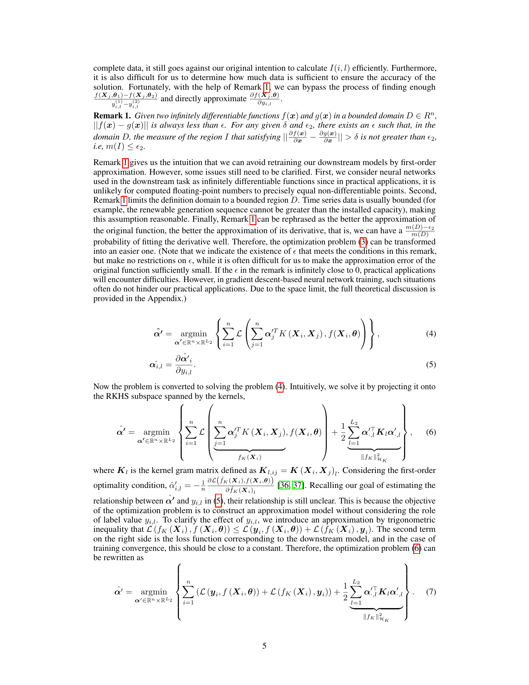
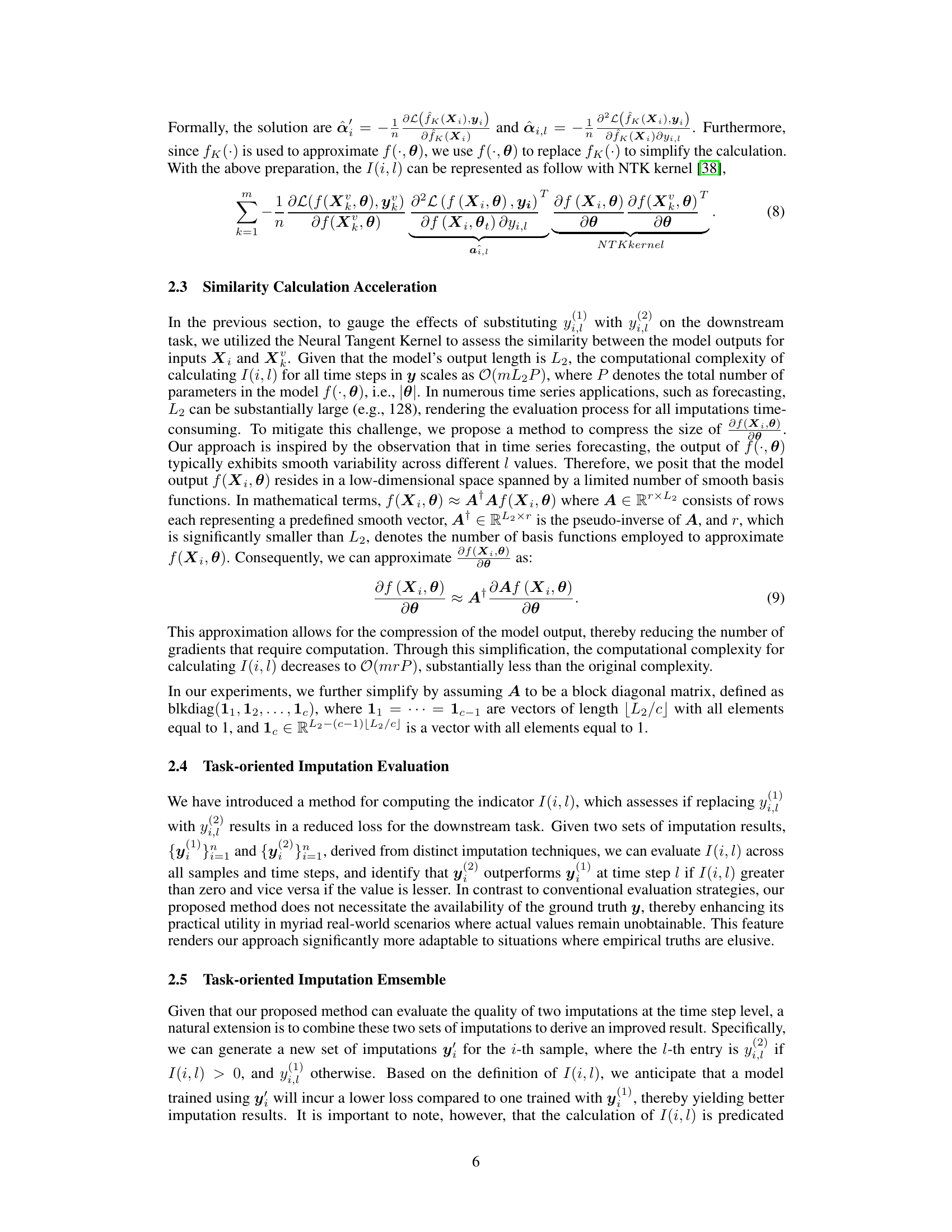
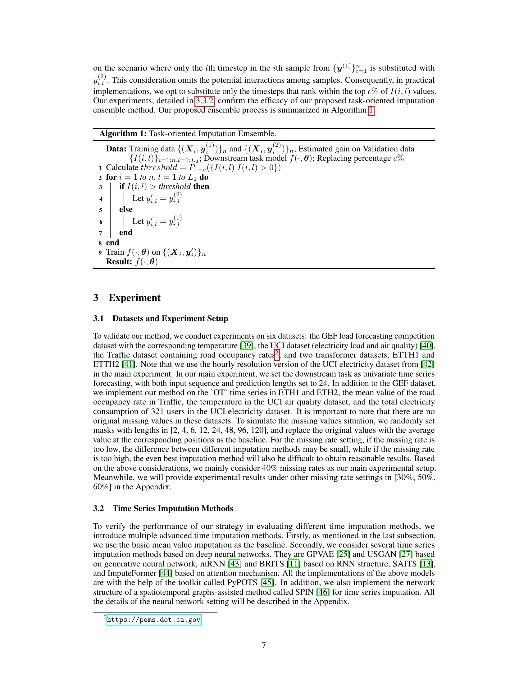
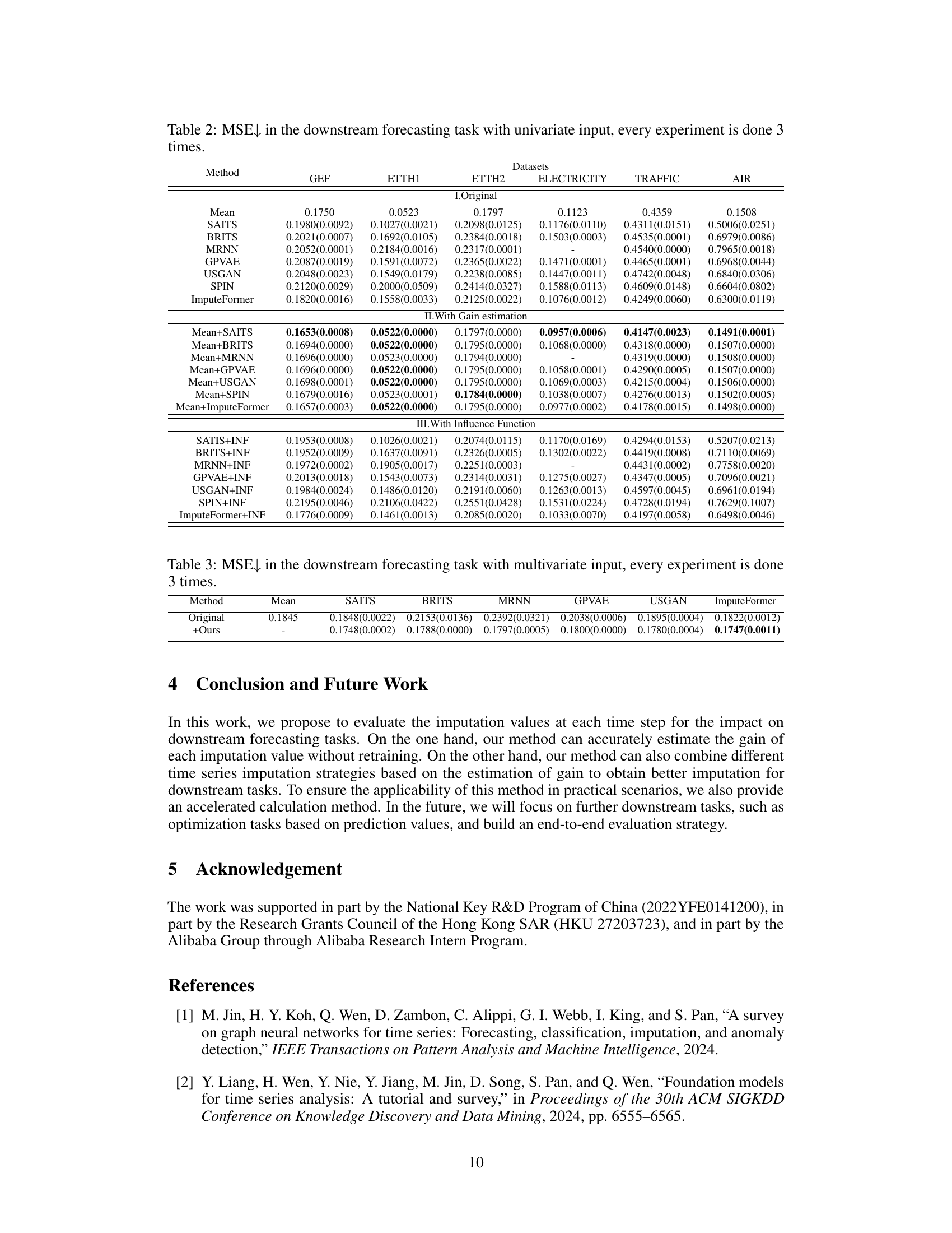
🔼 The figure compares the correlation and accuracy of three methods for estimating the gain of imputation for each time step. The methods are the original method, a modified influence function, and a segmented acceleration method. The x-axis shows the percentage of samples selected based on the estimated gain, while the y-axis shows the correlation and accuracy of the gain estimation.
read the caption
Figure 1: The correlation and accuracy comparison between the estimation of imputation value gain and actual gain (MSE↓), where INF (section D.5) represents our modified Influence Function, Seq-sim represents our original method, and Seg-N represents the acceleration method divided by N segments. The horizontal axis here represents selecting the sample with the highest x% influence based on the absolute value of the estimation.

🔼 This table compares the computation time of different methods for estimating the gain of imputation. The methods compared are Seq-sim (original method), Seg-4, Seg-2, Seg-1 (accelerated methods with different numbers of segments), and Retraining (retraining the forecasting model multiple times for each time step). The table shows that the accelerated methods significantly reduce computation time compared to retraining, with Seg-1 being the fastest among the accelerated methods. The time is measured in seconds (s).
read the caption
Table 1: Time comparison between different methods.
In-depth insights#
Task-Oriented Imputation#
Task-oriented imputation is a novel approach to handling missing data in time series by focusing on the downstream task’s performance. Instead of solely aiming for accurate imputation of missing values, this method directly evaluates imputation strategies based on how well they improve the results of the subsequent task (e.g., forecasting). This is particularly beneficial because an imputation method that excels in reconstructing missing values may not necessarily yield the best performance in the subsequent task. This task-oriented approach avoids unnecessary retraining of models for different imputation methods and significantly improves efficiency. The core idea is to estimate the gains of various imputation techniques for each time step without retraining and then combine them strategically to achieve optimal results for the specific downstream task. This approach effectively addresses the limitations of traditional methods that prioritize imputation accuracy over task performance, making it a significant advancement in handling missing data in time series analysis.
Representer Approach#
A representer theorem offers a powerful framework for simplifying complex machine learning models by showing that optimal solutions lie within a smaller, more manageable subspace. This is particularly valuable in tackling time series imputation, a challenging problem where data is often incomplete or noisy. By leveraging a representer theorem, one can reduce the computational burden associated with searching through a vast space of possible imputations. The choice of representer is crucial, impacting the model’s accuracy and efficiency. Generalized representers provide flexibility, enabling the combination of different imputation methods to optimize performance in downstream tasks. This task-oriented approach is key, as simple imputation accuracy does not guarantee success in practical applications. The efficiency of this approach relies on clever approximations, reducing the computational cost associated with repeated model retraining for each imputation evaluation.
Gain Estimation#
Gain estimation, in the context of time series imputation, is a crucial step that determines the effectiveness of imputation methods. It goes beyond simply assessing the accuracy of imputed values by focusing on how the imputed values improve downstream task performance, such as forecasting or classification. A key challenge is efficiently estimating these gains without repeatedly retraining models for each imputation strategy, which can be computationally expensive. The proposed approach tackles this challenge by employing a novel strategy that leverages the gradients of the downstream task to approximate the performance change caused by altering imputed values. This approximation cleverly avoids costly model retraining, providing a faster and more efficient way to evaluate imputation techniques. The method estimates the impact of each time step’s imputation on the downstream task, offering a fine-grained analysis of the imputation’s efficacy. It balances computational efficiency with accuracy. By incorporating this gain estimation, researchers can strategically combine imputation methods to obtain even better results than any single technique alone, maximizing the accuracy of downstream tasks. The efficiency and accuracy of this method are key advantages over traditional methods that only focus on the raw accuracy of imputation values.
Imputation Ensemble#
Imputation ensemble methods aim to leverage the strengths of multiple imputation techniques to improve the overall accuracy and robustness of missing data handling in time series analysis. The core idea is that combining diverse imputation strategies can mitigate the weaknesses of individual approaches. For example, one method might excel at imputing missing values in smooth regions, while another performs better with noisy or irregular data. By combining the results of multiple methods using a principled approach, the ensemble aims to produce imputations that are more accurate than any single method on its own. The effectiveness of an ensemble approach hinges on the diversity of the base imputers and the quality of the combination strategy. A poorly chosen combination method can lead to a less accurate imputation than the best individual imputer, while a strong combination strategy can result in substantial improvements in downstream tasks that rely on the imputed data. Therefore, the evaluation of ensemble methods should consider not only the immediate imputation quality but also its impact on these downstream tasks. This is crucial because the final goal is not just to fill in missing values but to use the imputed data to produce reliable and accurate results for prediction, anomaly detection, or other time series analysis applications.
Future Works#
The paper’s “Future Works” section would ideally expand upon its current task-oriented imputation method in several key areas. Extending the framework to encompass more diverse downstream tasks beyond forecasting, such as anomaly detection and classification, is crucial for broader applicability. A deeper investigation into the impact of different missing data mechanisms on imputation performance and the development of more robust imputation strategies tailored to specific types of missingness would enhance its practical value. Furthermore, exploring more advanced imputation methods, including those leveraging generative models or transformers, and integrating them into the task-oriented framework would be beneficial. Finally, a thorough exploration of the method’s scalability and computational efficiency for handling extremely large time series datasets, including potential optimizations and parallelization techniques, is necessary for real-world deployment. Addressing these aspects would solidify the paper’s contribution and significantly expand its impact on the time series imputation field.
More visual insights#
More on figures
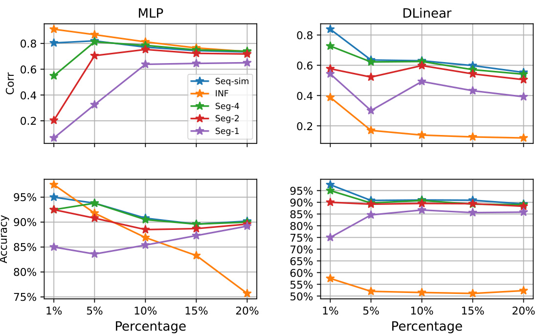
🔼 This figure compares the estimated gains of imputation for each time step using different methods against actual gains, using the Mean Squared Error (MSE) as the metric. The methods compared are the proposed method (Seq-sim), a modified influence function (INF), and accelerated versions of the proposed method (Seg-N, where N is the number of segments). The x-axis represents the percentage of samples selected based on the absolute value of the estimated gain. The figure shows that the proposed method provides a good correlation and accuracy in estimating the gains across different percentages of samples selected.
read the caption
Figure 1: The correlation and accuracy comparison between the estimation of imputation value gain and actual gain (MSE↓), where INF (section D.5) represents our modified Influence Function, Seq-sim represents our original method, and Seg-N represents the acceleration method divided by N segments. The horizontal axis here represents selecting the sample with the highest x% influence based on the absolute value of the estimation.
🔼 The figure shows the correlation and accuracy between the estimated and actual gains of imputation methods. The estimation uses three different approaches: the original method, a modified influence function, and a segmented acceleration method (with varying numbers of segments). The x-axis represents the percentage of samples selected based on the estimated gain magnitude.
read the caption
Figure 1: The correlation and accuracy comparison between the estimation of imputation value gain and actual gain (MSE↓), where INF (section D.5) represents our modified Influence Function, Seq-sim represents our original method, and Seg-N represents the acceleration method divided by N segments. The horizontal axis here represents selecting the sample with the highest x% influence based on the absolute value of the estimation.

🔼 The figure compares the correlation and accuracy of different methods for estimating the gain of imputation. The methods compared are the original method (Seq-sim), a modified influence function (INF), and an accelerated version of the original method divided into different numbers of segments (Seg-N). The x-axis represents the percentage of samples selected based on the estimated gain, while the y-axis represents both the correlation and accuracy of the gain estimation. The results indicate that the proposed method generally shows good performance, especially at higher percentages.
read the caption
Figure 1: The correlation and accuracy comparison between the estimation of imputation value gain and actual gain (MSE↓), where INF (section D.5) represents our modified Influence Function, Seq-sim represents our original method, and Seg-N represents the acceleration method divided by N segments. The horizontal axis here represents selecting the sample with the highest x% influence based on the absolute value of the estimation.

🔼 This figure compares the correlation and accuracy of different methods for estimating the gain of imputation. It shows how well the estimated gain correlates with the actual gain (measured by MSE reduction) and how accurately the method predicts the sign of the gain. Three methods are compared: the original method (Seq-sim), a modified influence function (INF), and an accelerated version of the original method (Seg-N, where N is the number of segments). The x-axis shows the percentage of samples selected based on the estimated gain magnitude.
read the caption
Figure 1: The correlation and accuracy comparison between the estimation of imputation value gain and actual gain (MSE↓), where INF (section D.5) represents our modified Influence Function, Seq-sim represents our original method, and Seg-N represents the acceleration method divided by N segments. The horizontal axis here represents selecting the sample with the highest x% influence based on the absolute value of the estimation.
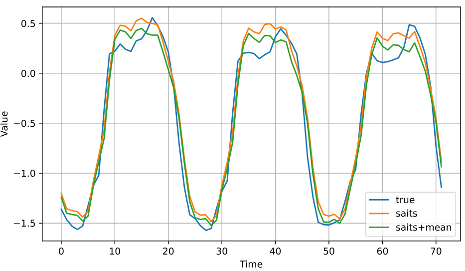
🔼 The figure compares the correlation and accuracy of different methods for estimating imputation value gains with actual gains. Three methods are compared: the original method, a modified Influence Function, and a segmented acceleration method. The x-axis represents the percentage of samples selected based on the estimated gain.
read the caption
Figure 1: The correlation and accuracy comparison between the estimation of imputation value gain and actual gain (MSE↓), where INF (section D.5) represents our modified Influence Function, Seq-sim represents our original method, and Seg-N represents the acceleration method divided by N segments. The horizontal axis here represents selecting the sample with the highest x% influence based on the absolute value of the estimation.

🔼 This figure compares the correlation and accuracy between the estimated and actual gains of imputation methods. The estimated gains are calculated using three different methods: the original method, a modified influence function, and a segmented acceleration method. The figure shows that the original method and the modified influence function have a high correlation, while the accuracy decreases as the percentage of estimated data increases for the influence function but remains high for the original method. The segmented acceleration method shows improved performance with increased segmentation.
read the caption
Figure 1: The correlation and accuracy comparison between the estimation of imputation value gain and actual gain (MSE↓), where INF (section D.5) represents our modified Influence Function, Seq-sim represents our original method, and Seg-N represents the acceleration method divided by N segments. The horizontal axis here represents selecting the sample with the highest x% influence based on the absolute value of the estimation.
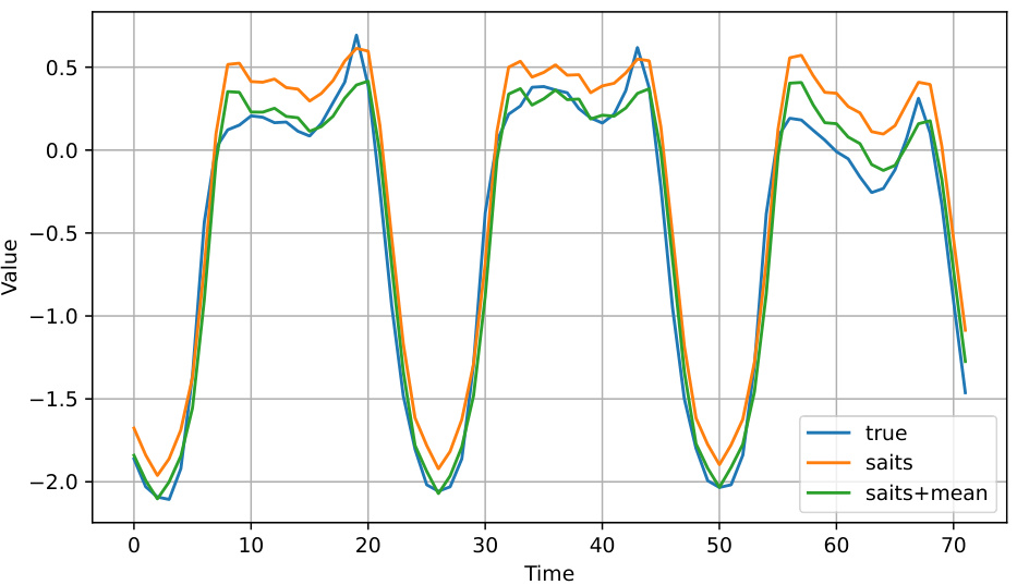
🔼 This figure compares the correlation and accuracy of the gain estimation methods against the actual gain (reduction in Mean Squared Error). It shows how well the different methods estimate the positive or negative impact of imputation on downstream forecasting tasks. The methods compared include the original method, a modified influence function, and the accelerated method with varying numbers of segments. The x-axis represents the percentage of top influential samples selected based on the absolute values of the estimated gains. The comparison assesses the accuracy of gain estimations for different methods.
read the caption
Figure 1: The correlation and accuracy comparison between the estimation of imputation value gain and actual gain (MSE↓), where INF (section D.5) represents our modified Influence Function, Seq-sim represents our original method, and Seg-N represents the acceleration method divided by N segments. The horizontal axis here represents selecting the sample with the highest x% influence based on the absolute value of the estimation.
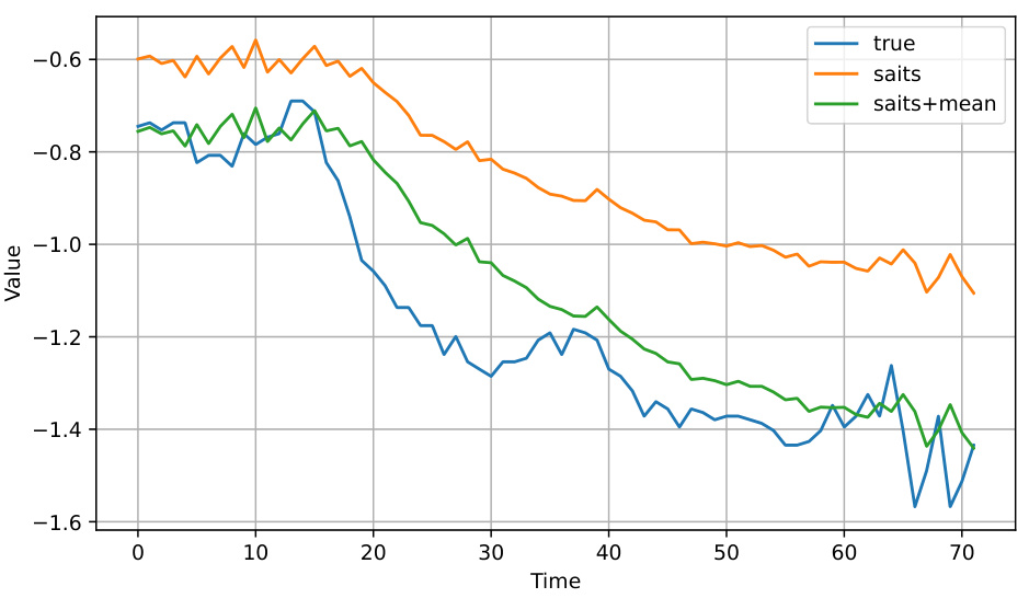
🔼 This figure compares the correlation and accuracy of estimating imputation value gains against actual gains (measured by Mean Squared Error reduction). Three methods are compared: the original method (Seq-sim), a modified Influence Function (INF), and a segmented acceleration method (Seg-N, where N represents the number of segments). The x-axis shows the percentage of samples selected for imputation based on the estimated gain. The results show the correlation and accuracy of estimating gains for different methods.
read the caption
Figure 1: The correlation and accuracy comparison between the estimation of imputation value gain and actual gain (MSE↓), where INF (section D.5) represents our modified Influence Function, Seq-sim represents our original method, and Seg-N represents the acceleration method divided by N segments. The horizontal axis here represents selecting the sample with the highest x% influence based on the absolute value of the estimation.

🔼 The figure compares the correlation and accuracy of different methods for estimating the gain of imputation. The methods compared are the original method (Seq-sim), a modified influence function (INF), and variations of an accelerated method (Seg-N, where N is the number of segments). The x-axis shows the percentage of samples selected based on estimated gain.
read the caption
Figure 1: The correlation and accuracy comparison between the estimation of imputation value gain and actual gain (MSE↓), where INF (section D.5) represents our modified Influence Function, Seq-sim represents our original method, and Seg-N represents the acceleration method divided by N segments. The horizontal axis here represents selecting the sample with the highest x% influence based on the absolute value of the estimation.
More on tables

🔼 This table presents the Mean Squared Error (MSE) results for six different datasets (GEF, ETTH1, ETTH2, ELECTRICITY, TRAFFIC, and AIR) across three different experimental setups. The first setup uses the original imputation methods. The second setup combines each original method with a proposed gain estimation method for improved performance. The third setup combines each original imputation method with an Influence Function technique. Lower MSE values indicate better performance.
read the caption
Table 2: MSE↓ in the downstream forecasting task with univariate input, every experiment is done 3 times.

🔼 This table presents the Mean Squared Error (MSE) for various time series imputation methods on six datasets when used in a univariate time series forecasting task. The MSE is a measure of the difference between the model’s predictions and the actual values. Lower MSE values indicate better performance. The table compares the performance of using the original imputation method versus methods that combine different imputation methods using the proposed gain estimation strategy. Results are shown for several different imputation methods, including SAITS, BRITS, MRNN, GPVAE, USGAN, and ImputeFormer. The table is divided into three sections: the original imputation performance, performance with gain estimation, and performance when using an Influence Function for label influence.
read the caption
Table 2: MSE↓ in the downstream forecasting task with univariate input, every experiment is done 3 times.

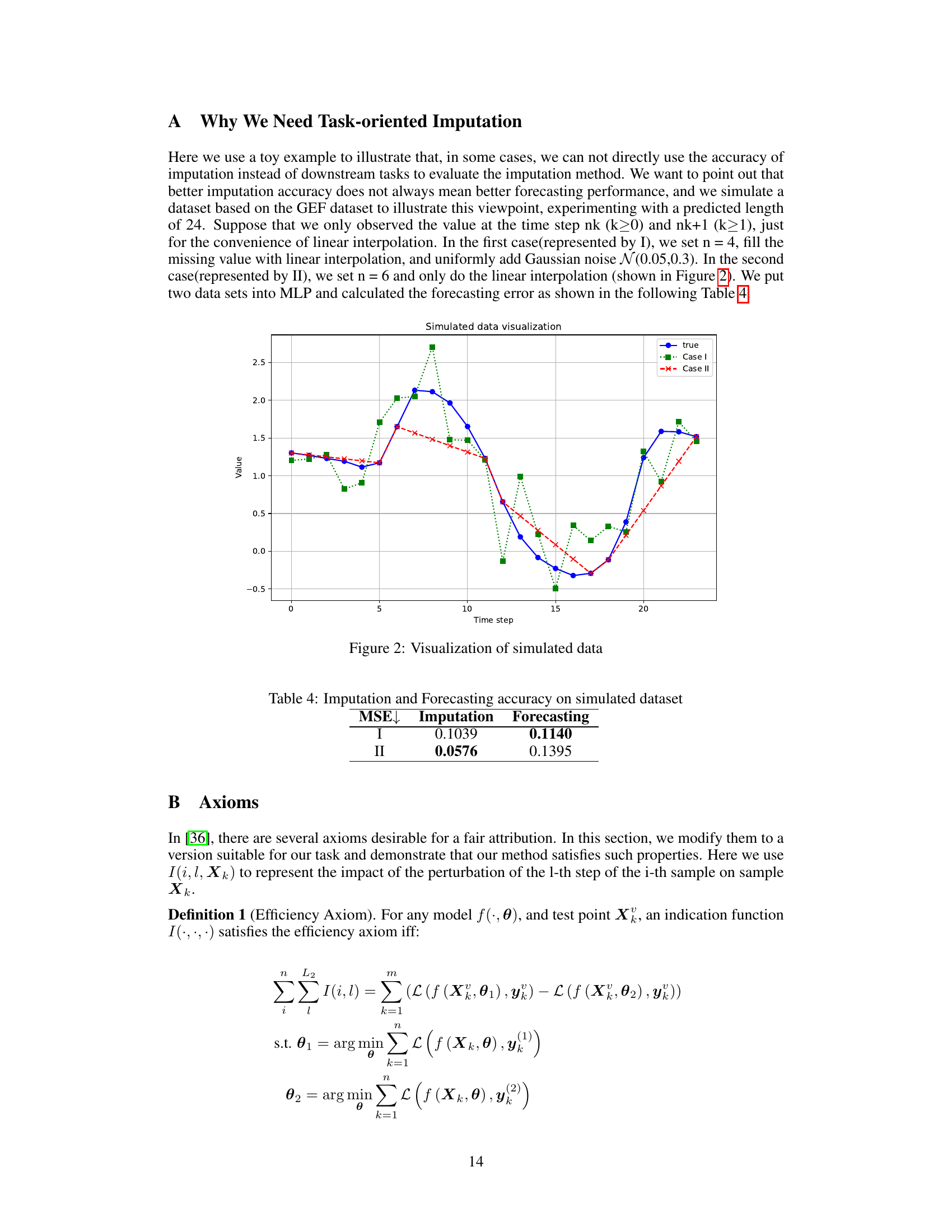
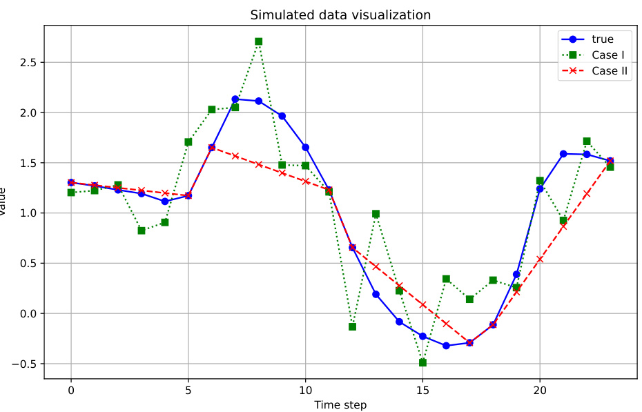
🔼 This table presents the Mean Squared Error (MSE) for both imputation and forecasting tasks on a simulated dataset. Two different scenarios (I and II) are compared. Scenario I involves filling missing values with linear interpolation and adding Gaussian noise, while scenario II uses only linear interpolation with a larger n value. The results demonstrate that lower imputation MSE does not always translate to better forecasting performance.
read the caption
Table 4: Imputation and Forecasting accuracy on simulated dataset

🔼 This table presents the Mean Squared Error (MSE) results for a univariate time series forecasting task across six different datasets. Multiple imputation methods are compared, both individually and when combined with the proposed gain estimation method. The table showcases the impact of the proposed method on improving forecasting accuracy across various datasets and imputation methods.
read the caption
Table 2: MSE↓ in the downstream forecasting task with univariate input, every experiment is done 3 times.

🔼 This table presents the Mean Squared Error (MSE) results for different time series imputation methods on six datasets. The MSE is a measure of the accuracy of the downstream forecasting task. Each imputation method was applied to the datasets and the MSE for each method and dataset was calculated. The lower the MSE, the better the performance of the imputation method in improving forecasting accuracy. The table is split into three sections: Original, With Gain estimation, and With Influence Function. The ‘Original’ section displays the MSE when the forecasting model is trained using the original dataset without imputation. The other sections show the improvements in MSE by using the proposed Gain estimation method and the Influence Function method, respectively.
read the caption
Table 2: MSE↓ in the downstream forecasting task with univariate input, every experiment is done 3 times.

🔼 This table presents the Mean Squared Error (MSE) results for the downstream forecasting task using various imputation methods. Univariate input was used and each experiment was repeated three times to enhance reliability. The table compares the original MSE values from different imputation methods (Mean, SAITS, BRITS, MRNN, GPVAE, USGAN, SPIN, ImputeFormer) with those obtained after applying the proposed gain estimation method combined with the original methods (Mean+SAITS, etc.) and compares both of them to those obtained using an influence function approach. The lower the MSE, the better the performance.
read the caption
Table 2: MSE↓ in the downstream forecasting task with univariate input, every experiment is done 3 times.

🔼 This table presents the Mean Squared Error (MSE) and computation time for different imputation methods on a larger dataset (the 15-minute resolution UCI electricity dataset), demonstrating the performance of the proposed method and its accelerated variants on a larger scale compared to the original method and other state-of-the-art methods.
read the caption
Table 8: MSE↓ comparison on larger dataset.

🔼 This table presents the Mean Squared Error (MSE) results for different time series imputation methods on the ELECTRICITY dataset with varying missing data rates (30%, 50%, and 60%). It compares the performance of the baseline (Mean imputation) to several advanced imputation methods (SAITS, BRITS, GPVAE, USGAN, ImputeFormer), both individually and when combined with the proposed gain-based imputation strategy (+ours). Lower MSE values indicate better imputation performance. The values in parentheses represent standard deviations across three independent trials.
read the caption
Table 9: MSE↓ comparison on different missing rate.

🔼 This table presents the Mean Squared Error (MSE) results for the downstream forecasting task using different time series imputation methods. Univariate input data is used. Each experiment is repeated three times to provide an indication of variability. The table compares the performance of various imputation methods alone (original) and the improvement obtained by combining the mean imputation with other methods (with gain estimation). A third section shows the impact of using an Influence Function to remove the most detrimental timesteps before forecasting.
read the caption
Table 2: MSE↓ in the downstream forecasting task with univariate input, every experiment is done 3 times.

🔼 This table presents the Mean Squared Error (MSE) results for a downstream forecasting task using multivariate input data. Multiple imputation methods (Mean, SAITS, BRITS, GPVAE, USGAN, ImputeFormer) are compared, showing their MSE values with and without the proposed task-oriented imputation ensemble method. The experiment was repeated three times to ensure reliable results. Lower MSE values indicate better performance.
read the caption
Table 3: MSE↓ in the downstream forecasting task with multivariate input, every experiment is done 3 times.
Full paper#
