TL;DR#
Working memory (WM), crucial for intelligent decisions, has been mainly studied using simplified inputs. Most research focuses on single tasks, leaving a gap in understanding how complex, real-world information is handled. This limits the generalizability of existing WM models and their biological plausibility.
This study used RNNs and naturalistic stimuli to address this gap by training them on multiple N-back tasks. The results showed RNNs maintain both relevant and irrelevant information simultaneously. Interestingly, object representation geometry showed that object features are less orthogonalized in the RNNs’ hidden space than in perceptual space. Crucially, the study demonstrates that RNNs utilize chronological memory subspaces to handle information over time, supporting resource-based models of WM rather than the classic slot-based model.
Key Takeaways#
Why does it matter?#
This paper is crucial for researchers in cognitive science and neural networks. It challenges existing models of working memory by using naturalistic stimuli and multi-task learning, offering novel insights into how brains manage complex information. The findings on chronological memory subspaces and representational geometry open new avenues for developing more realistic and biologically plausible models. This work is highly relevant to current trends in artificial intelligence and neuroscience, advancing our understanding of cognitive processes.
Visual Insights#

🔼 This figure details the experimental setup and model architecture used in the study. Panel (a) shows an example of a 2-back category task, where the model must determine if the category of the current stimulus matches that of the stimulus presented two steps earlier. Panel (b) outlines the various N-back task variations used, manipulating the number of steps back (N) and the type of object feature (location, identity, category). Panel (c) illustrates the two-stage sensory-cognitive model architecture, composed of a convolutional neural network (CNN) for visual processing and a recurrent neural network (RNN) for cognitive tasks. Panel (d) provides a schematic representation of how object properties (category, identity, location) are encoded and maintained in the model’s different latent subspaces (perceptual, encoding, memory). The figure illustrates how the model processes information through these subspaces during the tasks.
read the caption
Figure 1: Tasks and Models: a) Example of a 2-back category task. Each object's category is compared with the category of the object seen two frames prior. b) The suite of n-back tasks considered in the study. c) The sensory-cognitive model architecture. d) A schematic showing the latent subspaces for category, identity, and locations in the perceptual, encoding, and memory subspaces. Left: Stimuli are encoded in high dimensional latent space of the vision model (CNN). Each object property is encoded in a high dimensional latent subspace of this model; Right: RNN model represents each object property in its encoding latent subspace and retains some or all of the properties within its memory subspaces at later time points.
In-depth insights#
Naturalistic WM#
The concept of “Naturalistic WM” suggests a paradigm shift in working memory research. Traditional studies often rely on simplified, abstract stimuli, limiting the ecological validity of findings. A naturalistic approach, however, would involve using ecologically relevant, complex stimuli, thereby better reflecting real-world cognitive experiences. This necessitates investigating WM under more dynamic and task-demanding conditions. This approach aims to bridge the gap between laboratory-based tasks and real-life cognitive challenges. Researchers exploring this area would likely employ advanced neural network models trained on naturalistic datasets to better understand how the brain handles multi-dimensional information during complex cognitive tasks. The ultimate goal is to unravel how WM manages high-dimensional sensory information in the context of real-world tasks. Research in this area could have important implications for understanding cognitive impairment and developing more effective training and therapeutic interventions. By studying working memory with complex stimuli, researchers can uncover a deeper understanding of its capabilities and limitations, offering a more comprehensive view of this vital cognitive process.
RNN Task Geom#
Analyzing RNN task geometry reveals how recurrent neural networks represent and manipulate information during tasks. The organization of the RNN’s latent space directly reflects task demands, with task-relevant information more prominently encoded than irrelevant details. Interestingly, the study reveals that the degree of orthogonalization (separation) of object features within the RNN latent space is less than in the perceptual space, suggesting that RNNs employ less separated feature representations than expected. This is particularly true in gated RNNs (like GRUs and LSTMs), which exhibit more task-specific latent subspaces compared to vanilla RNNs. The results also highlight the crucial role of chronological memory subspaces in the N-back task, indicating that RNNs leverage temporal organization to track information effectively over short time intervals. This finding supports resource-based models of working memory. The transformations governing memory encoding and maintenance appear consistent across stimuli but are dynamic over time, suggesting flexible, adaptive mechanisms within the RNNs for managing information.
Multi-task RNNs#
The study investigates the capabilities of multi-task recurrent neural networks (RNNs) in handling naturalistic object representations within a working memory paradigm. A key finding highlights the simultaneous encoding of both task-relevant and irrelevant information in these RNNs, demonstrating a more holistic processing approach than previously thought. The research also delves into how RNN architectures, specifically gated vs. gateless models, influence the representation of object properties, revealing differences in the degree of task-specificity. Gated RNNs like GRUs and LSTMs exhibit greater task-specific latent subspaces, while gateless RNNs demonstrate more shared representations across tasks. This suggests that the choice of RNN architecture significantly affects the flexibility and generalizability of working memory models. Furthermore, the study sheds light on the nature of memory encoding and retention in RNNs, proposing a chronological memory subspace model to explain the temporal organization of information. This model contrasts with traditional slot-based WM models, suggesting a more dynamic and flexible capacity for information maintenance. The results offer valuable insights into the computational mechanisms underlying working memory and provide testable predictions for future neural studies.
Chronological WM#
The concept of “Chronological WM” suggests that working memory (WM) organizes information based on its temporal order of acquisition. This contrasts with models proposing separate memory slots or fixed-capacity buffers. The temporal organization allows for efficient encoding and retrieval, particularly in dynamic tasks like the N-back test, where information must be continuously updated and compared to incoming stimuli. Instead of relying on independent slots, chronological WM emphasizes the relative timing of information. Therefore, the model suggests that accessing older memories might involve traversing a temporal sequence of memory traces, rather than retrieving from a pre-defined location. This approach challenges traditional WM models that are often based on static representations, suggesting instead a more fluid and dynamic process deeply interwoven with time. This “chronological” aspect may also explain how the brain handles interfering information and distractions. It suggests that the temporal context is critical in maintaining the integrity of individual memory items, and that memory stability is not simply a property of individual memory slots but rather of their sequential relationships.
Future Research#
Future research directions stemming from this work could explore several key areas. Extending the investigation to other working memory tasks beyond the N-back paradigm would enhance the generalizability of the findings. It would be crucial to investigate the impact of task complexity and the number of items to be remembered on the observed representational patterns and orthogonality. Exploring the influence of different network architectures (e.g., transformers, attention mechanisms) could also provide insights into the range of computational strategies employed for WM. Additionally, a systematic comparison of different stimuli (e.g., images, sounds) is needed to assess the robustness of the findings across sensory modalities. Finally, bridging the gap between computational models and neurobiological data through rigorous comparisons with neural recordings would validate the theoretical model and provide testable predictions about the neural underpinnings of working memory.
More visual insights#
More on figures

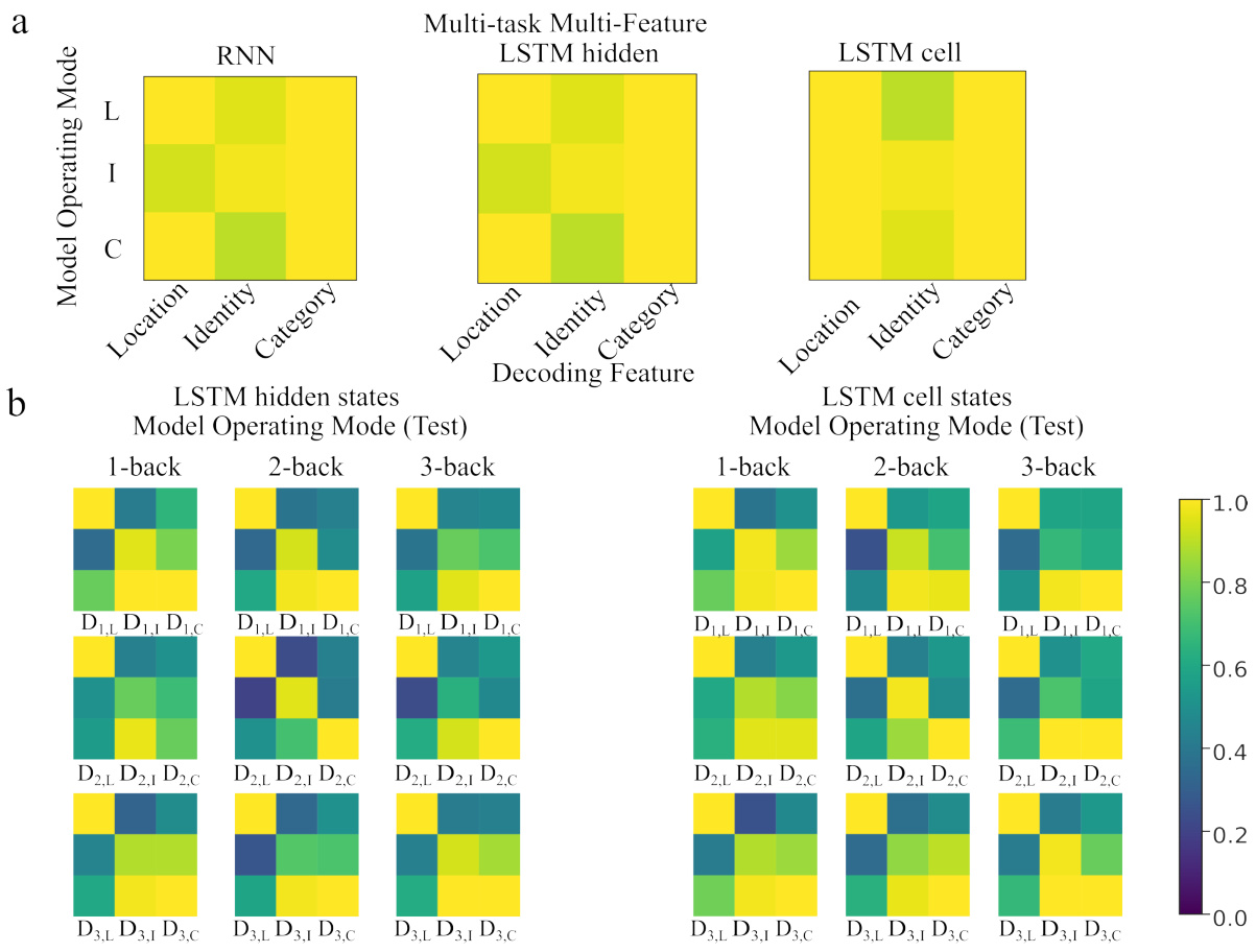
🔼 This figure displays the results of decoding analyses to assess how well RNNs represent task-relevant and task-irrelevant object properties. Panel (a) shows the generalization performance of decoders trained on one task and tested on others, revealing task specificity. Panel (b) shows decoding accuracy for specific object features, highlighting the ability of RNNs to retrieve task-relevant information. Panel (c) quantifies both within-task and cross-task decoding accuracies for different RNN architectures.
read the caption
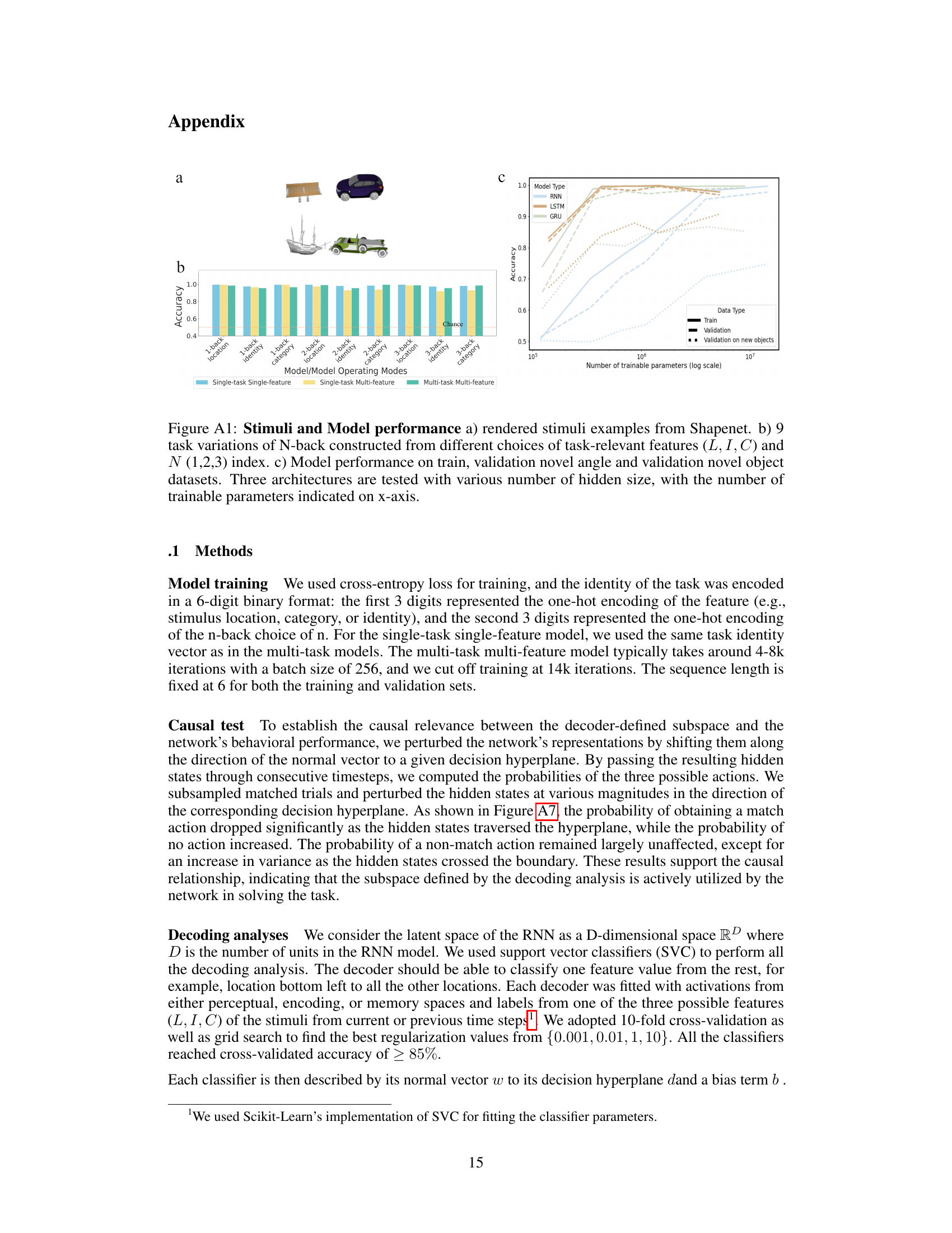
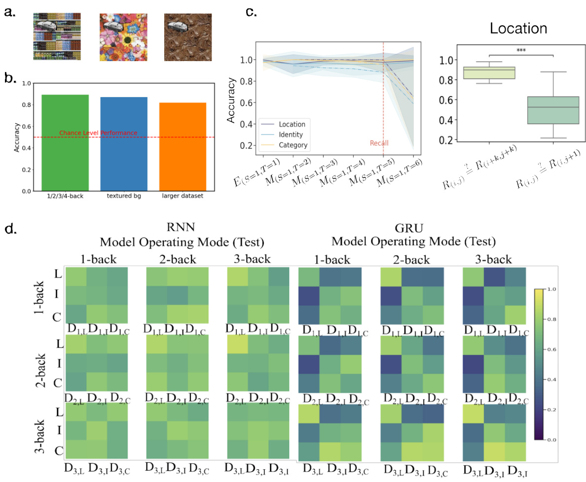
Figure 2: Representation of task-relevant/-irrelevant object properties: (a) Decoding generalization accuracy for each object property is displayed across tasks and operating modes for vanilla RNN and GRU. Rows and columns of 3 × 3 matrices correspond to the N-back task on which the decoders are fitted and tested on respectively. Matrix columns correspond to particular decoders denoted by Dk,F (k ∈ {1,2,3}, F ∈ {L, I, C'}) (indicating which task and decoding feature the decoder was fitted on), while matrix rows correspond to the object property of the task the decoder was tested on. (b) Validation accuracy of decoders trained on RNN latent space activations from the first time step of each trial to predict different object properties. Each column represents the object property the decoder was trained on, while each row corresponds to a model. c) Quantification of the validation accuracy (within the same task, indicated in purple) and generalization accuracy (across tasks with different task-relevant features, indicated in yellow) across all model architectures.

🔼 This figure illustrates the concept of representational orthogonalization in the context of object properties (location, identity, category) within both perceptual and encoding spaces of a recurrent neural network (RNN). Panel (a) uses 3D schematics to show how orthogonalization affects the separation of object feature representations. Panel (b) presents quantitative analyses comparing orthogonalization levels in perceptual and RNN encoding spaces across different tasks (1-back, 2-back, 3-back). Box plots summarize the comparison, showing statistical significance using t-tests.
read the caption
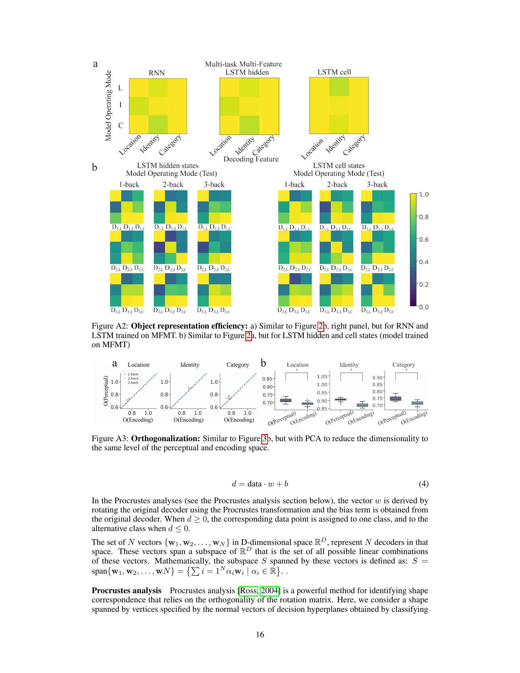
Figure 3: Orthogonalization: a) A schematic of two hypothetical object spaces in 3D. ri,j represents the angle formed by the decision hyperplanes that separate feature value i and j from each other. Top: non-orthogonalized representation; Bottom: orthogonalized representation. b) Upper panel: Normalized orthogonalization index, for both perceptual and encoding spaces respectively (denoted as O(Perceptual) and O(Encoding)). In most models, a less orthogonalized representation of feature values emerges in the RNN encoding space compared to the perceptual space (CNN output). Lower panel: Statistical comparison of the relative orthogonalization levels between the perceptual and encoding spaces. A two-sample t-test was performed to assess differences between the distributions of orthogonalization indices in the perceptual space and the encoding space.

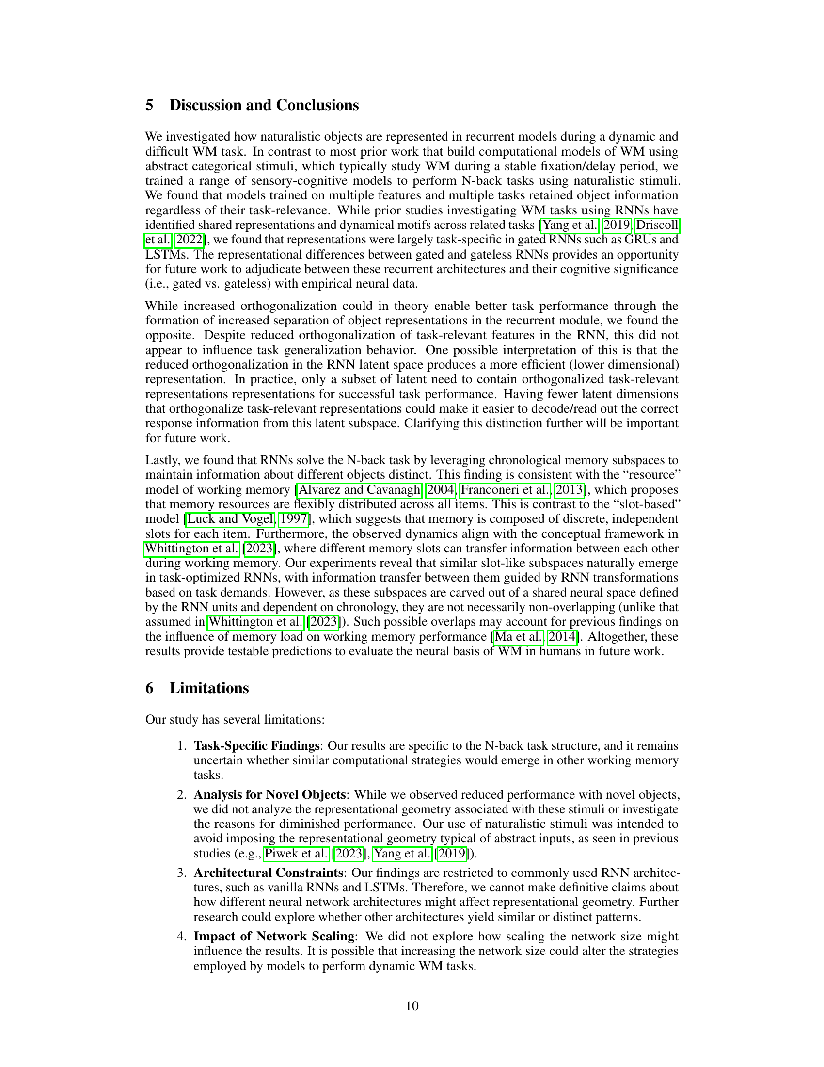
🔼 This figure shows how RNNs maintain information across time during a 3-back task. It demonstrates the encoding and memory subspaces used by the RNN, along with the transformations between them. The figure explores three hypotheses for how RNNs handle working memory and provides evidence supporting a chronological memory subspace model.
read the caption
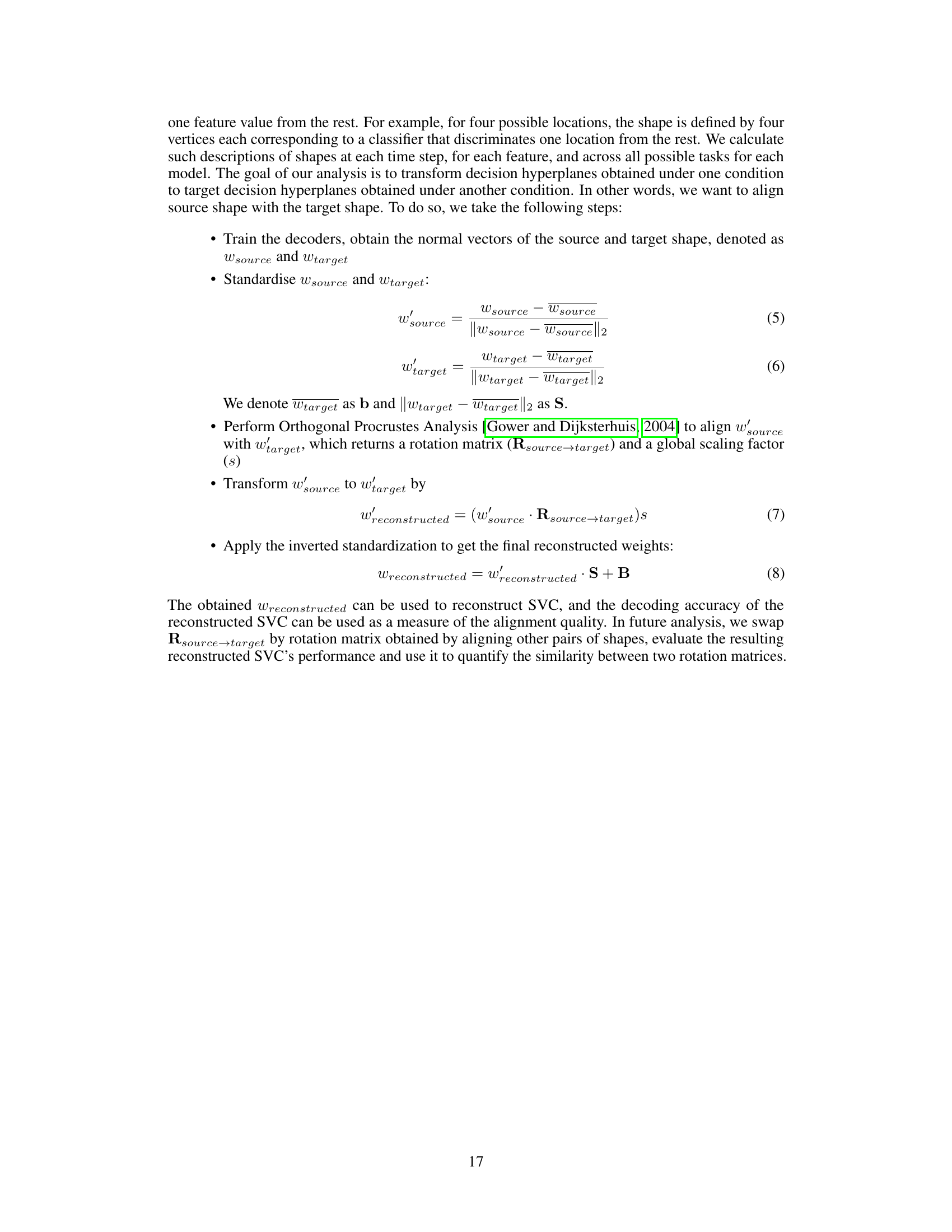
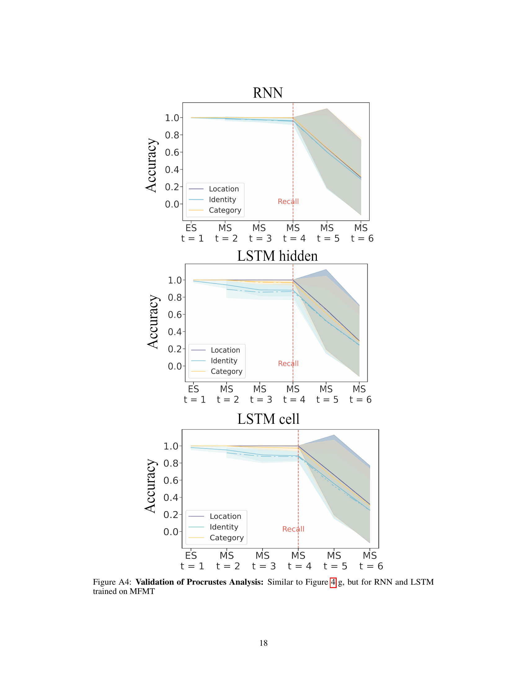
Figure 4: RNN dynamics during n-back task a) schematic of the 3-back task for a trial of 6 inputs. Model encodes each observed object in its respective Encoding Space denoted as E(i,j) (diagonal frames with yellow borders). For each stimulus, various object properties are retained over time in their respective Memory Space denoted as MS. On executive steps (frames with red borders) model produces a response according to the memory of the stimulus and the newly observed stimulus at that time. b) Decoding accuracy for predicting object identity at different time steps where the decoder is fit to data from the encoding step of a MTMF GRU during 1/2/3-back identity tasks. Red box indicates the executive steps. c) For each model type, we measured the generalization accuracy on executive (left boxplot) and non-executive (right boxplot) steps. d) Decoding accuracy for decoders trained and tested on the same Ei,i space (validation) or tested on other Ej,j,j ≠ i spaces. e) Schematic of the three hypotheses. f) Left: Schematic of the two latent space transformations. Structured transformation preserves the topology (i.e. the transformation can be captured solely by a common scaling factor and a rotation matrix). Unstructured transformation: does not preserve the topology. Right: Decoding accuracy for fitted decoders (solid line) and reconstructed decoders (dotted line) using the rotation matrix R(i,i) from the Procrustes analysis. The small accuracy gap between fitted and reconstructed decoders suggests a structured transformation. g) Decoding accuracy of the reconstructed decoder when the original rotation matrix is substituted with another (indicated by the x-axis labels). Rows and columns corresponds to object properties and MTMF network architectures respectively.

🔼 This figure illustrates the experimental setup and model architecture used in the study. Panel (a) shows an example of a 2-back category task, where the model must determine if the current stimulus matches the stimulus presented two steps earlier. Panel (b) presents an overview of all nine N-back tasks used, varying in the object properties (location, identity, category) and memory delay (N=1, 2, or 3). Panel (c) details the two-stage model architecture, consisting of a convolutional neural network (CNN) for visual processing and a recurrent neural network (RNN) for working memory. Panel (d) illustrates how object properties are encoded and maintained in the RNN’s latent space. The CNN encodes objects in a high-dimensional space, while the RNN maintains these features in task-specific subspaces, both across tasks and through time.
read the caption
Figure 1: Tasks and Models: a) Example of a 2-back category task. Each object's category is compared with the category of the object seen two frames prior. b) The suite of n-back tasks considered in the study. c) The sensory-cognitive model architecture. d) A schematic showing the latent subspaces for category, identity, and locations in the perceptual, encoding, and memory subspaces. Left: Stimuli are encoded in high dimensional latent space of the vision model (CNN). Each object property is encoded in a high dimensional latent subspace of this model; Right: RNN model represents each object property in its encoding latent subspace and retains some or all of the properties within its memory subspaces at later time points.
🔼 This figure illustrates the RNN’s dynamic behavior during the N-back task, focusing on how object information is encoded, maintained, and retrieved. It shows the latent subspaces used by the RNN, hypotheses on memory mechanisms, and the impact of transformations on the accuracy of reconstructed decoders.
read the caption
Figure 4: RNN dynamics during n-back task a) schematic of the 3-back task for a trial of 6 inputs. Model encodes each observed object in its respective Encoding Space denoted as E(i,j) (diagonal frames with yellow borders). For each stimulus, various object properties are retained over time in their respective Memory Space denoted as MS. On executive steps (frames with red borders) model produces a response according to the memory of the stimulus and the newly observed stimulus at that time. b) Decoding accuracy for predicting object identity at different time steps where the decoder is fit to data from the encoding step of a MTMF GRU during 1/2/3-back identity tasks. Red box indicates the executive steps. c) For each model type, we measured the generalization accuracy on executive (left boxplot) and non-executive (right boxplot) steps. d) Decoding accuracy for decoders trained and tested on the same Ei,i space (validation) or tested on other Ej,j,j ≠ i spaces. e) Schematic of the three hypotheses. f) Left: Schematic of the two latent space transformations. Structured transformation preserves the topology (i.e. the transformation can be captured solely by a common scaling factor and a rotation matrix). Unstructured transformation: does not preserve the topology. Right: Decoding accuracy for fitted decoders (solid line) and reconstructed decoders (dotted line) using the rotation matrix R(i,i) from the Procrustes analysis. The small accuracy gap between fitted and reconstructed decoders suggests a structured transformation. g) Decoding accuracy of the reconstructed decoder when the original rotation matrix is substituted with another (indicated by the x-axis labels). Rows and columns corresponds to object properties and MTMF network architectures respectively.

🔼 This figure demonstrates the concept of representational orthogonalization in the context of object feature encoding within RNNs. Panel (a) provides a visual illustration comparing orthogonalized and non-orthogonalized object representations in 3D space. Panel (b) presents a quantitative analysis of the degree of orthogonalization in both perceptual (CNN output) and encoding (RNN) spaces for location, identity, and category features, using boxplots to compare the orthogonalization indices between the two spaces. The comparison uses a two-sample t-test to assess statistical significance. In essence, the figure shows that RNN encodings have lower orthogonalization than perceptual spaces, suggesting a potentially more efficient encoding strategy.
read the caption
Figure 3: Orthogonalization: a) A schematic of two hypothetical object spaces in 3D. ri,j represents the angle formed by the decision hyperplanes that separate feature value i and j from each other. Top: non-orthogonalized representation; Bottom: orthogonalized representation. b) Upper panel: Normalized orthogonalization index, for both perceptual and encoding spaces respectively (denoted as O(Perceptual) and O(Encoding)). In most models, a less orthogonalized representation of feature values emerges in the RNN encoding space compared to the perceptual space (CNN output). Lower panel: Statistical comparison of the relative orthogonalization levels between the perceptual and encoding spaces. A two-sample t-test was performed to assess differences between the distributions of orthogonalization indices in the perceptual space and the encoding space.
🔼 This figure displays the RNN’s dynamic behavior during the N-back task. It illustrates the encoding and memory subspaces, showing how information is maintained and retrieved over time. The figure also proposes three hypotheses regarding the RNN’s memory mechanism and presents evidence supporting one of them, highlighting the use of chronological memory subspaces.
read the caption
Figure 4: RNN dynamics during n-back task a) schematic of the 3-back task for a trial of 6 inputs. Model encodes each observed object in its respective Encoding Space denoted as E(i,j) (diagonal frames with yellow borders). For each stimulus, various object properties are retained over time in their respective Memory Space denoted as MS. On executive steps (frames with red borders) model produces a response according to the memory of the stimulus and the newly observed stimulus at that time. b) Decoding accuracy for predicting object identity at different time steps where the decoder is fit to data from the encoding step of a MTMF GRU during 1/2/3-back identity tasks. Red box indicates the executive steps. c) For each model type, we measured the generalization accuracy on executive (left boxplot) and non-executive (right boxplot) steps. d) Decoding accuracy for decoders trained and tested on the same Ei,i space (validation) or tested on other Ej,j,j ≠ i spaces. e) Schematic of the three hypotheses. f) Left: Schematic of the two latent space transformations. Structured transformation preserves the topology (i.e. the transformation can be captured solely by a common scaling factor and a rotation matrix). Unstructured transformation: does not preserve the topology. Right: Decoding accuracy for fitted decoders (solid line) and reconstructed decoders (dotted line) using the rotation matrix R(i,i) from the Procrustes analysis. The small accuracy gap between fitted and reconstructed decoders suggests a structured transformation. g) Decoding accuracy of the reconstructed decoder when the original rotation matrix is substituted with another (indicated by the x-axis labels). Rows and columns corresponds to object properties and MTMF network architectures respectively.

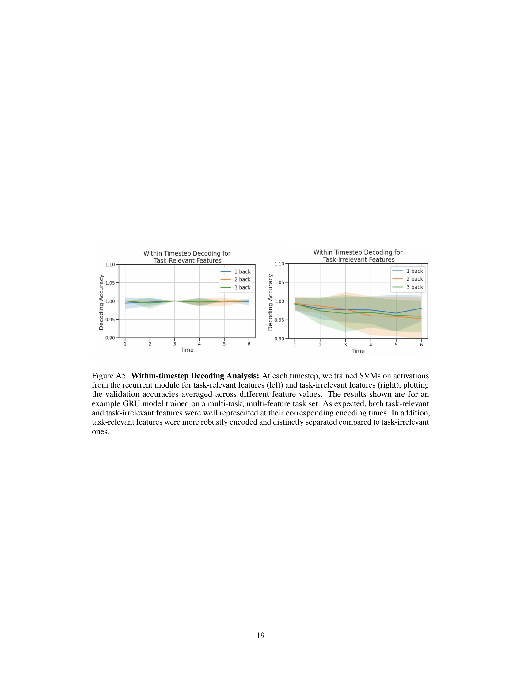
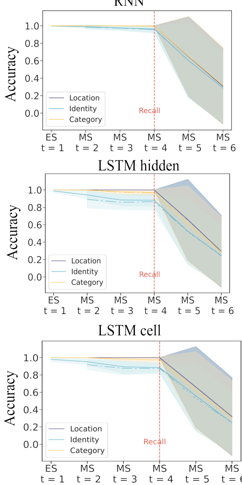
🔼 This figure shows the results of decoding analysis performed on a GRU model trained on multiple tasks and features. Two subplots are presented: one for task-relevant features and one for task-irrelevant features. The y-axis represents decoding accuracy, and the x-axis represents time. The shaded regions indicate the standard deviation of the accuracy across various trials. The results show that task-relevant features are more accurately decoded than task-irrelevant features, with higher accuracy for task-relevant features consistently maintained over time.
read the caption
Figure A5: Within-timestep Decoding Analysis: At each timestep, we trained SVMs on activations from the recurrent module for task-relevant features (left) and task-irrelevant features (right), plotting the validation accuracies averaged across different feature values. The results shown are for an example GRU model trained on a multi-task, multi-feature task set. As expected, both task-relevant and task-irrelevant features were well represented at their corresponding encoding times. In addition, task-relevant features were more robustly encoded and distinctly separated compared to task-irrelevant ones.
🔼 This figure summarizes the RNN’s dynamic behavior during the N-back task. It illustrates how the model encodes and retains object information across time steps, distinguishing between encoding and memory spaces. It shows the decoding accuracies for predicting object properties across different stages of the task, and explores the hypotheses for different memory subspace mechanisms. The orthogonal Procrustes analysis is used to quantify the transformation between the representation spaces.
read the caption
Figure 4: RNN dynamics during n-back task a) schematic of the 3-back task for a trial of 6 inputs. Model encodes each observed object in its respective Encoding Space denoted as E(i,j) (diagonal frames with yellow borders). For each stimulus, various object properties are retained over time in their respective Memory Space denoted as MS. On executive steps (frames with red borders) model produces a response according to the memory of the stimulus and the newly observed stimulus at that time. b) Decoding accuracy for predicting object identity at different time steps where the decoder is fit to data from the encoding step of a MTMF GRU during 1/2/3-back identity tasks. Red box indicates the executive steps. c) For each model type, we measured the generalization accuracy on executive (left boxplot) and non-executive (right boxplot) steps. d) Decoding accuracy for decoders trained and tested on the same Ei,i space (validation) or tested on other Ej,j,j ≠ i spaces. e) Schematic of the three hypotheses. f) Left: Schematic of the two latent space transformations. Structured transformation preserves the topology (i.e. the transformation can be captured solely by a common scaling factor and a rotation matrix). Unstructured transformation: does not preserve the topology. Right: Decoding accuracy for fitted decoders (solid line) and reconstructed decoders (dotted line) using the rotation matrix R(i,i) from the Procrustes analysis. The small accuracy gap between fitted and reconstructed decoders suggests a structured transformation. g) Decoding accuracy of the reconstructed decoder when the original rotation matrix is substituted with another (indicated by the x-axis labels). Rows and columns corresponds to object properties and MTMF network architectures respectively.

🔼 This figure illustrates the RNN’s dynamic behavior during the N-back task. It breaks down the model’s encoding and memory processes, showing how it handles task-relevant and irrelevant information, and how it utilizes memory subspaces over time. The figure also compares different hypotheses about how RNNs implement the N-back task, and it explores the transformations between encoding and memory spaces.
read the caption
Figure 4: RNN dynamics during n-back task a) schematic of the 3-back task for a trial of 6 inputs. Model encodes each observed object in its respective Encoding Space denoted as E(i,j) (diagonal frames with yellow borders). For each stimulus, various object properties are retained over time in their respective Memory Space denoted as MS. On executive steps (frames with red borders) model produces a response according to the memory of the stimulus and the newly observed stimulus at that time. b) Decoding accuracy for predicting object identity at different time steps where the decoder is fit to data from the encoding step of a MTMF GRU during 1/2/3-back identity tasks. Red box indicates the executive steps. c) For each model type, we measured the generalization accuracy on executive (left boxplot) and non-executive (right boxplot) steps. d) Decoding accuracy for decoders trained and tested on the same Ei,i space (validation) or tested on other Ej,j,j ≠ i spaces. e) Schematic of the three hypotheses. f) Left: Schematic of the two latent space transformations. Structured transformation preserves the topology (i.e. the transformation can be captured solely by a common scaling factor and a rotation matrix). Unstructured transformation: does not preserve the topology. Right: Decoding accuracy for fitted decoders (solid line) and reconstructed decoders (dotted line) using the rotation matrix R(i,i) from the Procrustes analysis. The small accuracy gap between fitted and reconstructed decoders suggests a structured transformation. g) Decoding accuracy of the reconstructed decoder when the original rotation matrix is substituted with another (indicated by the x-axis labels). Rows and columns corresponds to object properties and MTMF network architectures respectively.
Full paper#


