TL;DR#
Current counterfactual reasoning methods often generate unrealistic scenarios due to their non-backtracking nature. This limits their applicability and usefulness. This paper addresses this challenge by proposing “natural counterfactuals”, which incorporates a controlled amount of backtracking to find more realistic scenarios while prioritizing the least amount of changes needed. This approach involves a novel optimization that balances backtracking and naturalness.
The proposed method utilizes an optimization framework that balances backtracking with a ’naturalness’ criterion. Experiments on synthetic and real-world datasets demonstrate that natural counterfactuals significantly reduce prediction errors compared to existing approaches, showcasing their ability to learn more effectively from real-world data and provide more reliable insights in various application scenarios. The framework is especially beneficial in high-stake applications involving machine learning. The improved feasibility of generated counterfactuals enhances the reliability of predictions and the usefulness of the method in practical settings.
Key Takeaways#
Why does it matter?#
This paper is important because it introduces a novel approach to counterfactual reasoning, a crucial area of AI research with applications in various fields. The proposed method addresses limitations of existing approaches by incorporating necessary backtracking, leading to more realistic and reliable counterfactual scenarios. This opens up new avenues for research in explainable AI, causal inference, and decision-making systems.
Visual Insights#

🔼 This figure visualizes the results of the proposed method and the non-backtracking method on Toy 1 dataset. Subfigure (a) shows the outcome error on a single sample, highlighting the significant reduction in error achieved by the proposed method (0.03) compared to the non-backtracking method (2.31). Subfigure (b) presents a scatter plot showing the relationship between ground truth and prediction for n3, demonstrating that the proposed method’s predictions align more closely with the ground truth than the non-backtracking method.
read the caption
Figure 1: The Visualization Results on Toy 1 (View the enlarged figure in Fig. 3 in the Appendix).

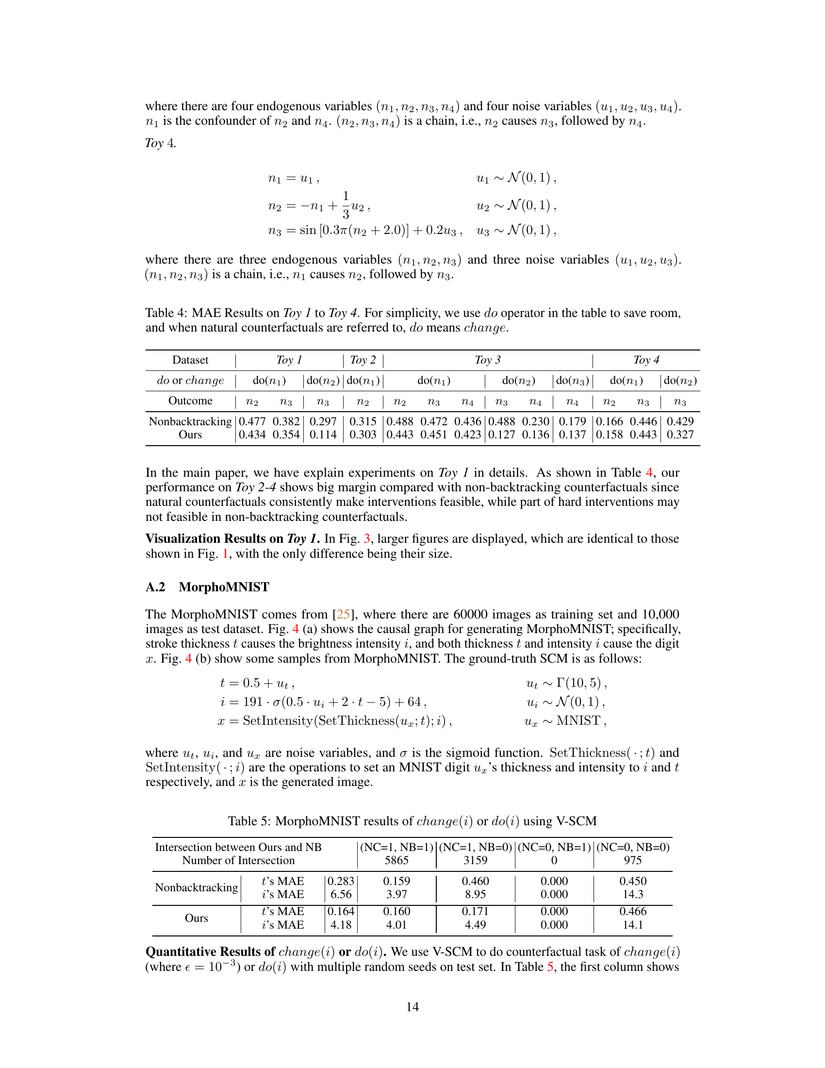
🔼 This table presents the Mean Absolute Error (MAE) results for four toy datasets (Toy 1 to Toy 4) comparing the performance of the proposed natural counterfactual method against a non-backtracking baseline. Lower MAE indicates better performance. The ‘do’ notation is used interchangeably with ‘change’ for natural counterfactuals to save space.
read the caption
Table 1: MAE Results on Toy 1 to Toy 4 (Lower MAE is better). To save room, we also write “do” for “change” for natural counterfactuals.
In-depth insights#
Natural CFs#
The concept of “Natural CFs” (Counterfactuals) presents a compelling alternative to traditional, non-backtracking counterfactual generation methods. The core idea is to allow for a degree of backtracking in causal reasoning, moving away from the strict surgical interventions of Pearl’s approach. This flexibility enables the generation of more realistic and plausible counterfactual scenarios that align better with observed data distributions. By incorporating a “naturalness” criterion and an optimization framework, the method carefully balances the need for backtracking with the goal of minimizing deviations from reality. This is particularly important for machine learning applications where out-of-distribution counterfactuals can lead to unreliable predictions. Empirical experiments demonstrate the effectiveness of this approach, showcasing improved accuracy and reliability compared to methods that solely rely on non-backtracking counterfactuals. However, a limitation is that this optimization process may not always have a solution, depending on the strictness of the naturalness criteria. The computational cost is another factor to consider. Despite these limitations, Natural CFs represent a significant advance in generating realistic and useful counterfactual explanations.
Backtracking#
The concept of backtracking in the context of counterfactual reasoning presents a nuanced approach to generating realistic and plausible scenarios. Unlike non-backtracking methods, which strictly adhere to causal pathways, backtracking allows for adjustments in causally preceding variables to minimize deviations from observed data distributions. This approach enhances the feasibility of counterfactual scenarios by ensuring they remain within the realm of realistic possibilities. A key advantage is the ability to learn from real-world data, addressing the limitations of non-backtracking methods that struggle to generate counterfactuals outside of the observed distribution. However, uncontrolled backtracking can lead to counterfactuals that are overly nuanced or unrealistic. Therefore, a critical aspect is the need for mechanisms to regulate the extent of backtracking, often employing optimization techniques to balance between realism and parsimony. This involves defining criteria that prioritize ’naturalness’ in counterfactuals, thus ensuring that adjustments remain within bounds of realistic data.
Feasible FIO#
The concept of “Feasible FIO” suggests a refinement of the original FIO (Feasible Intervention Optimization) framework, addressing its limitations. A key issue with FIO might be the generation of unrealistic counterfactuals, far removed from the observed data distribution. Feasible FIO likely incorporates mechanisms to ensure generated counterfactuals remain within a realistic range. This could involve incorporating constraints based on data density, employing statistical measures of naturalness, or other techniques to limit deviation from the training data. The optimization process might involve a trade-off: achieving the desired counterfactual change while minimizing deviations from the realistic scenarios. This focus on feasibility underscores a practical application of the method, making it more applicable to real-world datasets with limited coverage. The success of Feasible FIO hinges on the effectiveness of its naturalness criterion and the chosen distance metric for measuring deviations from observed data. It’s crucial that the methods for identifying feasible interventions are both theoretically sound and computationally efficient for practical use.
Empirical Results#
An effective ‘Empirical Results’ section in a research paper would begin by clearly stating the goals of the empirical study, aligning them with the paper’s overall hypotheses. The methodology used for data collection and analysis should be described precisely, including details on sample size, data sources, and statistical techniques. Results should be presented systematically, using tables and figures to clearly illustrate key findings and avoiding unnecessary jargon. Crucially, the discussion should move beyond simply reporting numbers; it should connect the results back to the hypotheses, offering clear interpretations and acknowledging any limitations or unexpected findings. Statistical significance should be explicitly addressed, indicating whether the findings are statistically significant and discussing potential confounding factors. Finally, a strong ‘Empirical Results’ section would provide a concise conclusion summarizing the key empirical findings and their implications for the paper’s claims, linking these results back to the broader field of study and outlining directions for future research. Robustness checks and sensitivity analyses are also important to assess the reliability and generalizability of results.
Future Work#
Future research directions stemming from this paper could explore several promising avenues. Extending the framework to handle more complex causal structures and scenarios with latent variables is crucial for broader applicability. Investigating alternative naturalness criteria and distance metrics, potentially incorporating domain-specific knowledge, could lead to more nuanced and effective counterfactual generation. A deeper theoretical analysis comparing and contrasting different notions of counterfactuals is warranted to better understand their strengths and limitations in various applications. Finally, developing more efficient algorithms and scaling the approach to handle massive datasets will be essential for real-world deployment. The potential ethical implications of generating counterfactuals, especially in high-stakes decision-making contexts, also deserve thorough consideration and further investigation.
More visual insights#
More on figures
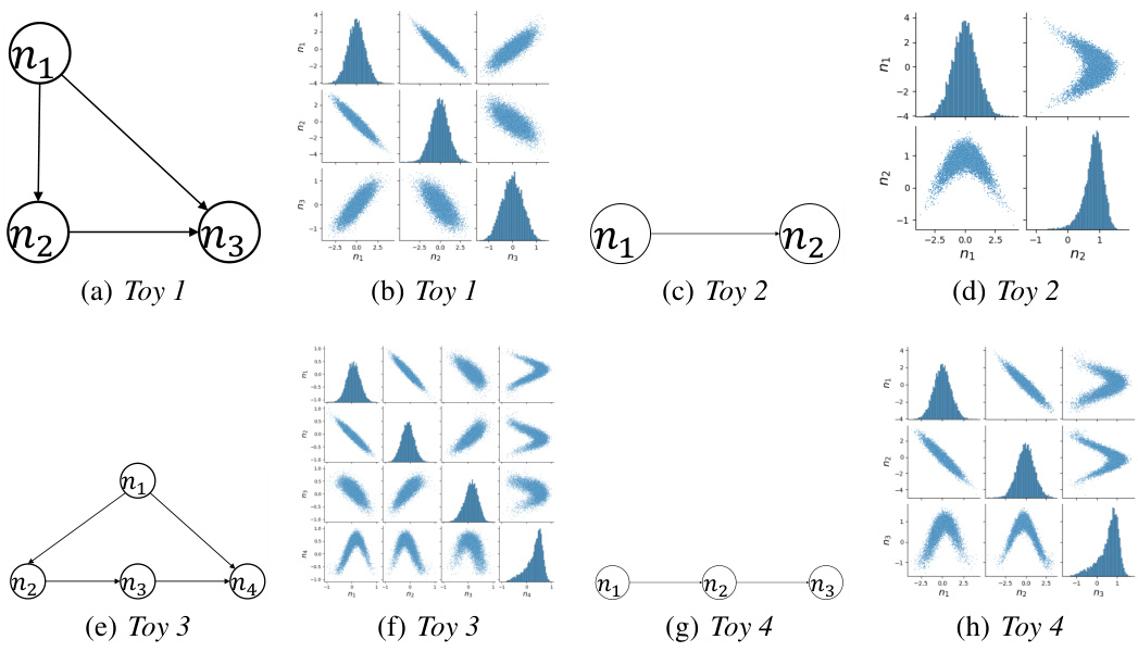
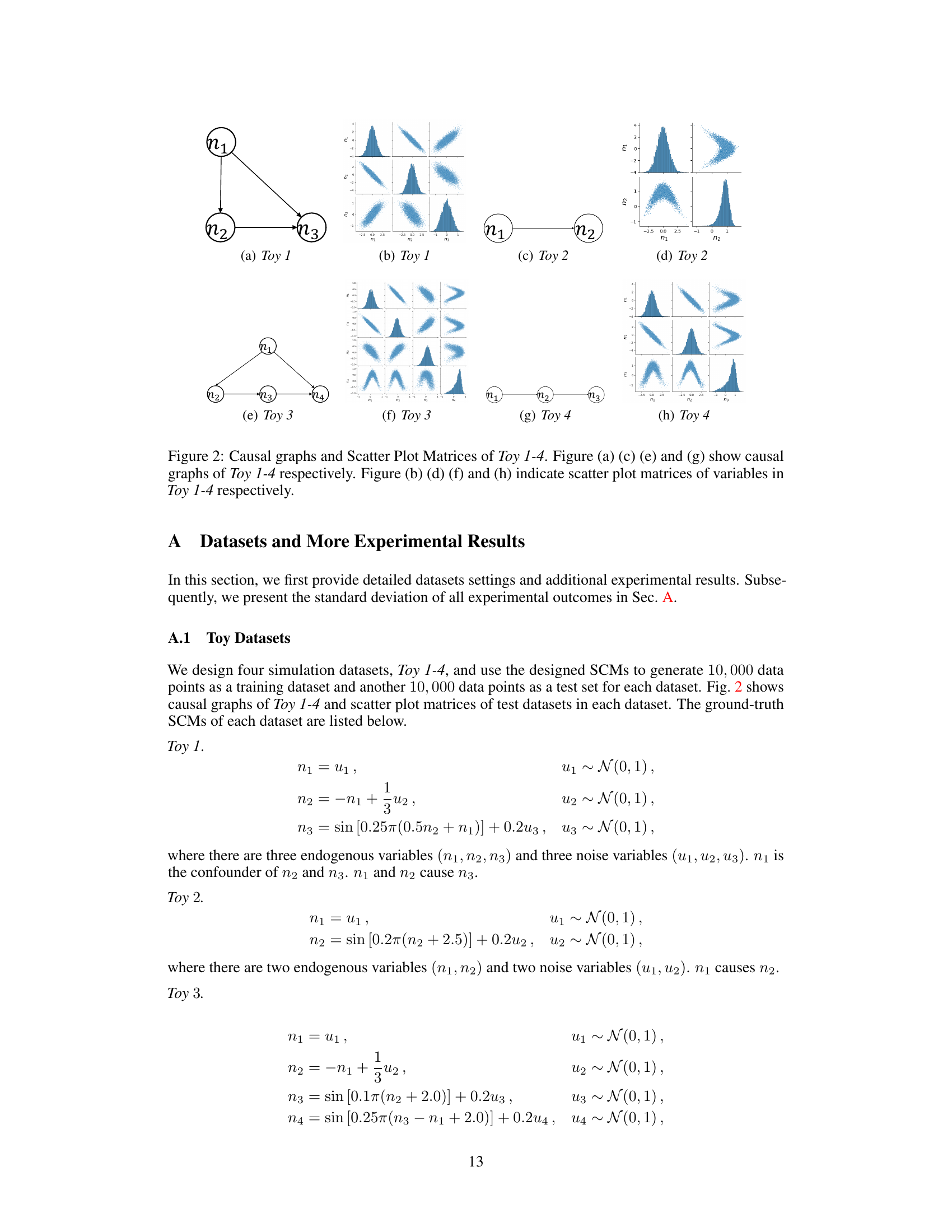
🔼 This figure visualizes the causal relationships and data distributions for four synthetic datasets (Toy 1-4) used in the paper’s experiments. The left column shows the causal graphs representing the relationships between variables in each dataset. The right column displays scatter plot matrices for each dataset, illustrating the joint distributions of the variables and providing a visual representation of their correlations and dependencies. These visualizations help in understanding the data characteristics and their suitability for evaluating the proposed counterfactual methods.
read the caption
Figure 2: Causal graphs and Scatter Plot Matrices of Toy 1-4. Figure (a) (c) (e) and (g) show causal graphs of Toy 1-4 respectively. Figure (b) (d) (f) and (h) indicate scatter plot matrices of variables in Toy 1-4 respectively.

🔼 This figure visualizes the results of a single sample from the Toy 1 dataset. It shows the effectiveness of the proposed natural counterfactual method compared to a non-backtracking approach. Panel (a) displays the outcome error on a single sample, highlighting how the natural counterfactual method significantly reduces error compared to the non-backtracking method. Panel (b) shows a scatter plot of ground truth versus predicted values for n3, illustrating the improved accuracy and alignment with the y=x line achieved using the natural counterfactual approach.
read the caption
Figure 1: The Visualization Results on Toy 1 (View the enlarged figure in Fig. 3 in the Appendix).

🔼 This figure visualizes the results of a single sample from the Toy 1 dataset, comparing the performance of natural counterfactuals and non-backtracking counterfactuals. Panel (a) shows the outcome error for a single sample, illustrating how natural counterfactuals significantly reduce the error compared to non-backtracking counterfactuals. Panel (b) presents a scatter plot comparing ground truth versus predictions for n3, highlighting the superior alignment of natural counterfactuals with the y=x line, indicating more accurate predictions.
read the caption
Figure 1: The Visualization Results on Toy 1 (View the enlarged figure in Fig. 3 in the Appendix).
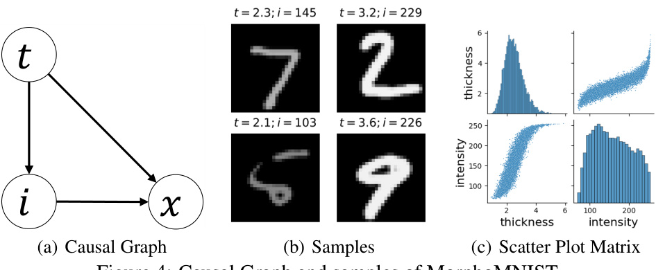
🔼 This figure shows the causal graph and some samples from the MorphoMNIST dataset. The causal graph depicts that the digit stroke thickness (t) influences both the brightness intensity (i) and the digit image (x), while the intensity (i) directly affects the image (x). The samples demonstrate different values of thickness (t) and intensity (i), and their corresponding generated images (x). Additionally, scatter plot matrices visualize the relationships between the variables.
read the caption
Figure 4: Causal Graph and samples of MorphoMNIST.

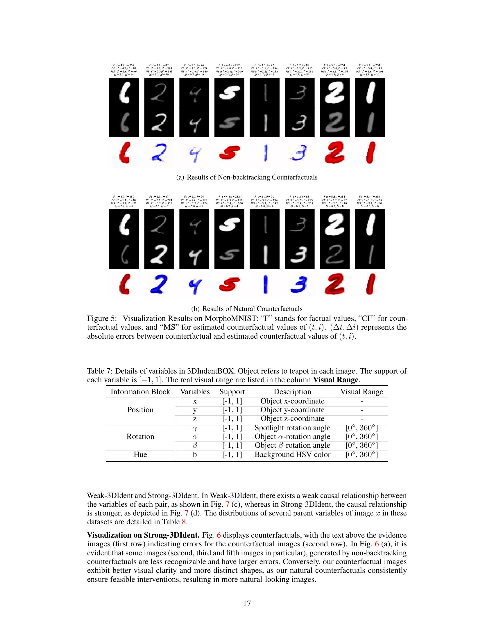
🔼 This figure visualizes the results of counterfactual generation on the MorphoMNIST dataset. It compares the factual values (F), the generated counterfactual values using the proposed method (CF), and the estimated values using the model (MS) for the thickness (t) and intensity (i) of digit strokes. The difference between the counterfactual (CF) and model-estimated (MS) values, (∆t, ∆i), is also shown. This highlights the accuracy and naturalness of the generated counterfactuals compared to a non-backtracking approach.
read the caption
Figure 5: Visualization Results on MorphoMNIST: “F” stands for factual values, “CF” for counterfactual values, and “MS” for estimated counterfactual values of (t, i). (∆t, ∆i) represents the absolute errors between counterfactual and estimated counterfactual values of (t, i).
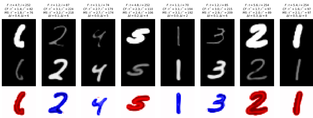
🔼 This figure visualizes the results of counterfactual generation on the MorphoMNIST dataset. It shows comparisons between the factual values (F), counterfactual values generated using the proposed method (CF), and those estimated from a predictive model (MS) for pairs of thickness (t) and intensity (i) in a sample of images. The differences between the counterfactual and model-estimated values (∆t, ∆i) are also displayed, providing a quantitative measure of the method’s accuracy. The results illustrate the effectiveness of the approach in producing natural, feasible counterfactuals that are close to the ground truth and easily recognizable, in contrast to non-backtracking counterfactual methods.
read the caption
Figure 5: Visualization Results on MorphoMNIST: “F” stands for factual values, “CF” for counterfactual values, and “MS” for estimated counterfactual values of (t, i). (∆t, ∆i) represents the absolute errors between counterfactual and estimated counterfactual values of (t, i).
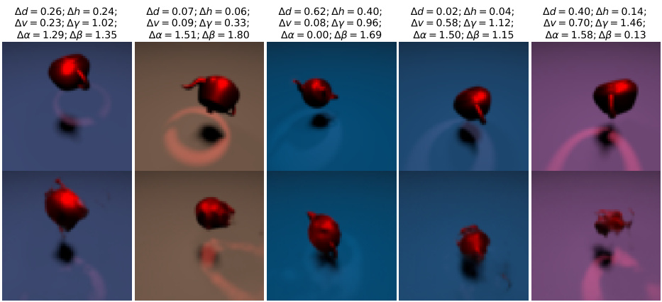
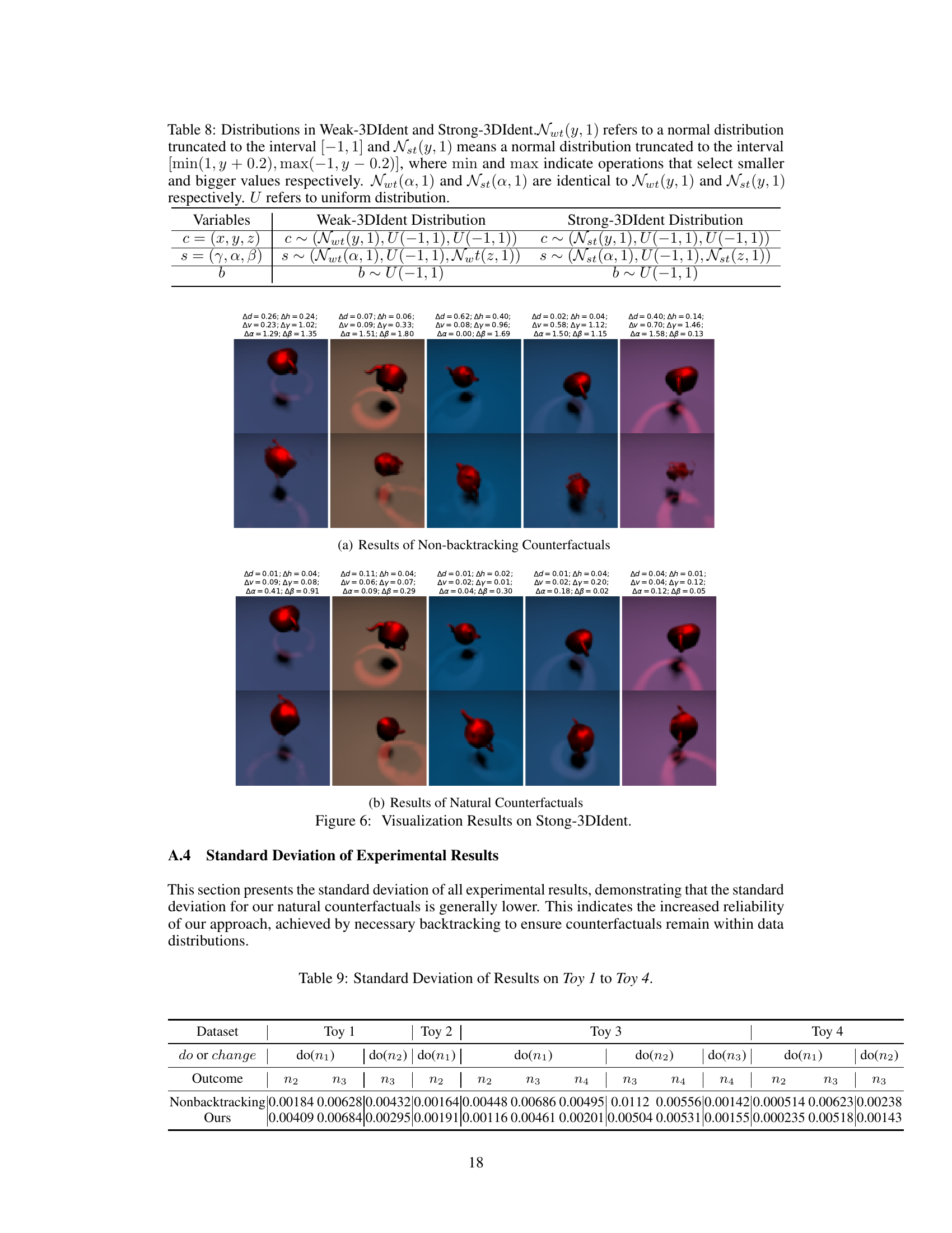
🔼 This figure visualizes the results of counterfactual generation on the Strong-3DIdent dataset. The top row shows the original images, while the bottom row shows the generated counterfactual images using both non-backtracking and natural counterfactual methods. The text above each image quantifies the differences between the original and counterfactual images using error metrics for various image attributes (Δd, Δh, Δv, Δγ, Δα, Δβ). The results show that the natural counterfactual method produces images that are more visually similar to the original images compared to the non-backtracking approach, highlighting its effectiveness in generating more natural and realistic counterfactual instances.
read the caption
Figure 6: Visualization Results on Stong-3DIdent.

🔼 This figure visualizes the results of both non-backtracking and natural counterfactual methods on the Strong-3DIdent dataset. The top row shows the original images, while the bottom row displays the generated counterfactual images. The text above each image in the top row indicates the absolute errors between the ground truth and the generated counterfactual values. The results demonstrate that the natural counterfactual approach produces visually more plausible and accurate results than the non-backtracking approach, particularly when dealing with more complex scenarios.
read the caption
Figure 6: Visualization Results on Stong-3DIdent.
🔼 This figure visualizes the causal relationships and data distributions for four synthetic datasets (Toy 1-4) used in the paper’s experiments. The left column shows the causal graphs, illustrating the dependencies between variables in each dataset. The right column presents scatter plot matrices which depict the joint distributions of the variables. These visualizations help understand the data characteristics and the underlying causal mechanisms for each dataset.
read the caption
Figure 2: Causal graphs and Scatter Plot Matrices of Toy 1-4. Figure (a) (c) (e) and (g) show causal graphs of Toy 1-4 respectively. Figure (b) (d) (f) and (h) indicate scatter plot matrices of variables in Toy 1-4 respectively.

🔼 This figure shows the causal graph and some sample images from the MorphoMNIST dataset. The causal graph depicts the relationships between the variables: thickness (t), intensity (i), and image (x). The sample images illustrate how variations in thickness and intensity affect the generated digit image.
read the caption
Figure 4: Causal Graph and samples of MorphoMNIST.
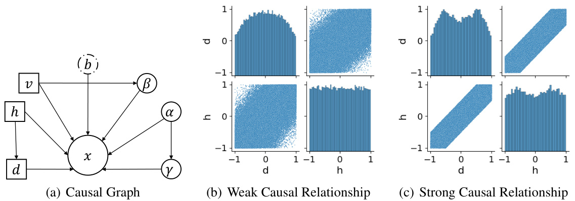
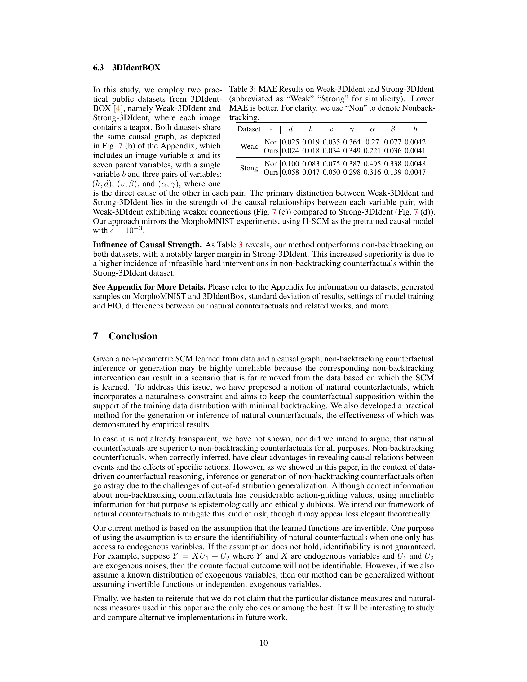
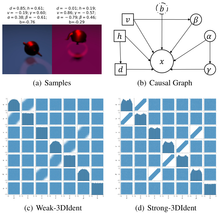
🔼 This figure visualizes the causal relationships between variables in the 3DIdentBOX dataset. Panel (a) shows the causal graph where variables d, h, v, γ, α, β, and b causally influence the image variable x. Panels (b) and (c) present scatter plot matrices for Weak-3DIdent and Strong-3DIdent, respectively, which showcase the difference in the strength of causal relationships between variable pairs (d, h), (v, β), and (α, γ) between the two datasets.
read the caption
Figure 7: Samples, Causal Graph, Scatter Plot Matrices of Weak-3DIdent and Strong-3DIdent.

🔼 This figure visualizes the results of counterfactual generation on the Strong-3DIdent dataset. The top row shows the original images (evidence). The bottom row displays the generated counterfactual images, with the text above each image indicating the error in the corresponding counterfactual outcomes. The results highlight the differences between natural counterfactuals (less error, more visually coherent images) and non-backtracking counterfactuals (more error, images that are less visually coherent and realistic).
read the caption
Figure 6: Visualization Results on Stong-3DIdent.
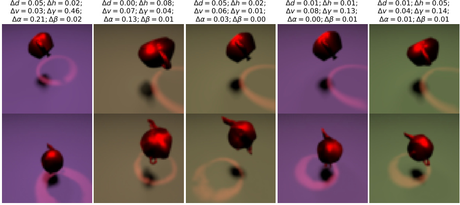
🔼 This figure visualizes the results of counterfactual generation on the Strong-3DIdent dataset. It compares the results of non-backtracking counterfactuals (a) with the proposed natural counterfactuals (b). Each row shows a set of images. The top row shows the original images (evidence). The middle row shows counterfactual images generated using each method. The bottom row displays the difference images between original and counterfactual images. The text above each image in the top row quantifies the changes (differences) in attributes using the non-backtracking and natural counterfactual methods. The results demonstrate that natural counterfactuals maintain more visually realistic and coherent images, unlike the non-backtracking counterfactuals which generate more distorted or unnatural-looking results.
read the caption
Figure 6: Visualization Results on Stong-3DIdent.
More on tables
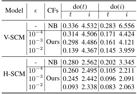
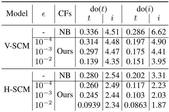
🔼 This table presents the results of an ablation study on the hyperparameter epsilon (e) used in the Feasible Intervention Optimization (FIO) framework. The study evaluates the impact of different epsilon values on the Mean Absolute Error (MAE) for both thickness (t) and intensity (i) across two different deep learning causal models, namely V-SCM and H-SCM. Lower MAE values indicate better performance. The table shows that as epsilon increases, the MAE generally decreases, suggesting that a stricter criterion for naturalness in counterfactual generation leads to better results.
read the caption
Table 2: Ablation Study on e (Lower MAE is better)

🔼 This table presents the Mean Absolute Error (MAE) results for four different toy datasets (Toy 1 to Toy 4). The MAE is a measure of the difference between the model’s predicted outcomes and the actual ground-truth outcomes for counterfactual scenarios. The table compares the performance of the proposed ’natural counterfactuals’ method with a standard non-backtracking approach. Lower MAE values indicate better performance. Note that in this table, ‘do’ is used as a shorthand for ‘change’ when referring to natural counterfactuals.
read the caption
Table 1: MAE Results on Toy 1 to Toy 4 (Lower MAE is better). To save room, we also write “do” for “change” for natural counterfactuals.

🔼 This table presents the Mean Absolute Error (MAE) results for four toy datasets (Toy 1 to Toy 4). Lower MAE values indicate better performance. The table compares the performance of the proposed ’natural counterfactuals’ approach with a traditional non-backtracking approach. The ‘do’ and ‘change’ notations are used interchangeably for natural counterfactuals, simplifying the table’s presentation.
read the caption
Table 1: MAE Results on Toy 1 to Toy 4 (Lower MAE is better). To save room, we also write “do” for “change” for natural counterfactuals.

🔼 This table presents the Mean Absolute Error (MAE) results for four different toy datasets (Toy 1 to Toy 4). It compares the performance of the proposed method (natural counterfactuals) against a non-backtracking approach. Lower MAE values indicate better performance. The ‘do’ abbreviation is used to represent both ‘do’ and ‘change’ operations for natural counterfactuals in this specific table for brevity.
read the caption
Table 1: MAE Results on Toy 1 to Toy 4 (Lower MAE is better). To save room, we also write “do” for “change” for natural counterfactuals.
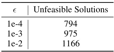
🔼 This table shows the number of unfeasible solutions encountered per 10,000 instances in the MorphoMNIST dataset for different values of the naturalness threshold (epsilon). An unfeasible solution occurs when the optimization problem in the Feasible Intervention Optimization (FIO) framework fails to find a solution that meets the naturalness criterion, even when the desired change is attainable. The results indicate that a stricter naturalness criterion (higher epsilon) leads to more unfeasible solutions, making it harder to find counterfactual scenarios consistent with the observed data distribution.
read the caption
Table 6: Unfeasible solutions per 10,000 instances on MorphoMNIST

🔼 This table presents the Mean Absolute Error (MAE) results for four different toy datasets (Toy 1 to Toy 4). The MAE measures the average absolute difference between predicted and ground truth outcomes for counterfactual scenarios. Lower MAE values indicate better performance. The table compares the performance of the proposed ’natural counterfactuals’ method against a standard non-backtracking approach. For natural counterfactuals, ‘do’ is used as a shorthand for ‘change’, reflecting that the desired change might be achieved by interventions on multiple upstream variables.
read the caption
Table 1: MAE Results on Toy 1 to Toy 4 (Lower MAE is better). To save room, we also write “do” for “change” for natural counterfactuals.

🔼 This table presents the Mean Absolute Error (MAE) results for four toy datasets (Toy 1 to Toy 4). It compares the performance of the proposed ’natural counterfactuals’ method against a non-backtracking approach. Lower MAE values indicate better performance. The ‘do’ notation is used as a shorthand for ‘change’ in the context of natural counterfactuals.
read the caption
Table 1: MAE Results on Toy 1 to Toy 4 (Lower MAE is better). To save room, we also write “do” for “change” for natural counterfactuals.

🔼 This table presents the Mean Absolute Error (MAE) results for four toy datasets (Toy 1 to Toy 4) comparing the proposed method for generating natural counterfactuals against a non-backtracking approach. Lower MAE indicates better performance. The ‘do’ notation is used as a shorthand for ‘change’ when referring to natural counterfactuals in this table.
read the caption
Table 1: MAE Results on Toy 1 to Toy 4 (Lower MAE is better). To save room, we also write “do” for “change” for natural counterfactuals.

🔼 This table presents the Mean Absolute Error (MAE) results for four toy datasets (Toy 1 to Toy 4) comparing the performance of the proposed natural counterfactual method against a non-backtracking baseline. Lower MAE indicates better performance. The ‘do’ notation is used interchangeably with ‘change’ for natural counterfactuals to save space.
read the caption
Table 1: MAE Results on Toy 1 to Toy 4 (Lower MAE is better). To save room, we also write “do” for “change” for natural counterfactuals.

🔼 This table presents the Mean Absolute Error (MAE) results for four different toy datasets (Toy 1 to Toy 4). The MAE measures the difference between the predicted and ground truth outcomes of counterfactual scenarios. Lower MAE values indicate better performance. The table compares the performance of the proposed method (denoted as ‘Ours’) against a non-backtracking method. Note that for natural counterfactuals, ‘do’ is used as a shorthand for ‘change’.
read the caption
Table 1: MAE Results on Toy 1 to Toy 4 (Lower MAE is better). To save room, we also write “do” for “change” for natural counterfactuals.

🔼 This table presents the Mean Absolute Error (MAE) results for four different toy datasets (Toy 1 to Toy 4). It compares the performance of the proposed ’natural counterfactuals’ method against a traditional ’non-backtracking’ approach for generating counterfactual instances. Lower MAE values indicate better performance. The ‘do’ notation is used as a shorthand for ‘change’ in the context of natural counterfactuals.
read the caption
Table 1: MAE Results on Toy 1 to Toy 4 (Lower MAE is better). To save room, we also write “do” for “change” for natural counterfactuals.

🔼 This table presents the Mean Absolute Error (MAE) results for four different toy datasets (Toy 1 to Toy 4). The MAE is a measure of the difference between predicted and actual outcomes for counterfactual scenarios. Two methods are compared: a non-backtracking approach and the proposed ’natural counterfactuals’ method. Lower MAE values indicate better performance. For brevity, ‘do’ is used as shorthand for ‘change’ in the natural counterfactuals column.
read the caption
Table 1: MAE Results on Toy 1 to Toy 4 (Lower MAE is better). To save room, we also write “do” for “change” for natural counterfactuals.
🔼 This table presents the Mean Absolute Error (MAE) results for four toy datasets (Toy1 to Toy4). Lower MAE indicates better performance. The table compares the performance of the proposed ’natural counterfactuals’ method with a standard non-backtracking approach. For natural counterfactuals, the abbreviation ‘do’ is used in place of ‘change’ to save space in the table.
read the caption
Table 1: MAE Results on Toy 1 to Toy 4 (Lower MAE is better). To save room, we also write “do” for “change” for natural counterfactuals.

🔼 This table presents the Mean Absolute Error (MAE) results for four toy datasets (Toy 1 to Toy 4). The MAE measures the deviation between the generated counterfactual outcomes and the ground truth outcomes. Lower MAE values indicate better performance. The table compares the performance of the proposed method (Ours) against a non-backtracking method (Nonbacktracking) for different intervention targets (n1, n2, n3, etc.) within each toy dataset. The ‘do’ notation represents both ‘change’ operations in the natural counterfactuals, indicating that natural counterfactuals allow for backtracking when necessary to ensure the counterfactual scenario remains realistic.
read the caption
Table 1: MAE Results on Toy 1 to Toy 4 (Lower MAE is better). To save room, we also write “do” for “change” for natural counterfactuals.
Full paper#


