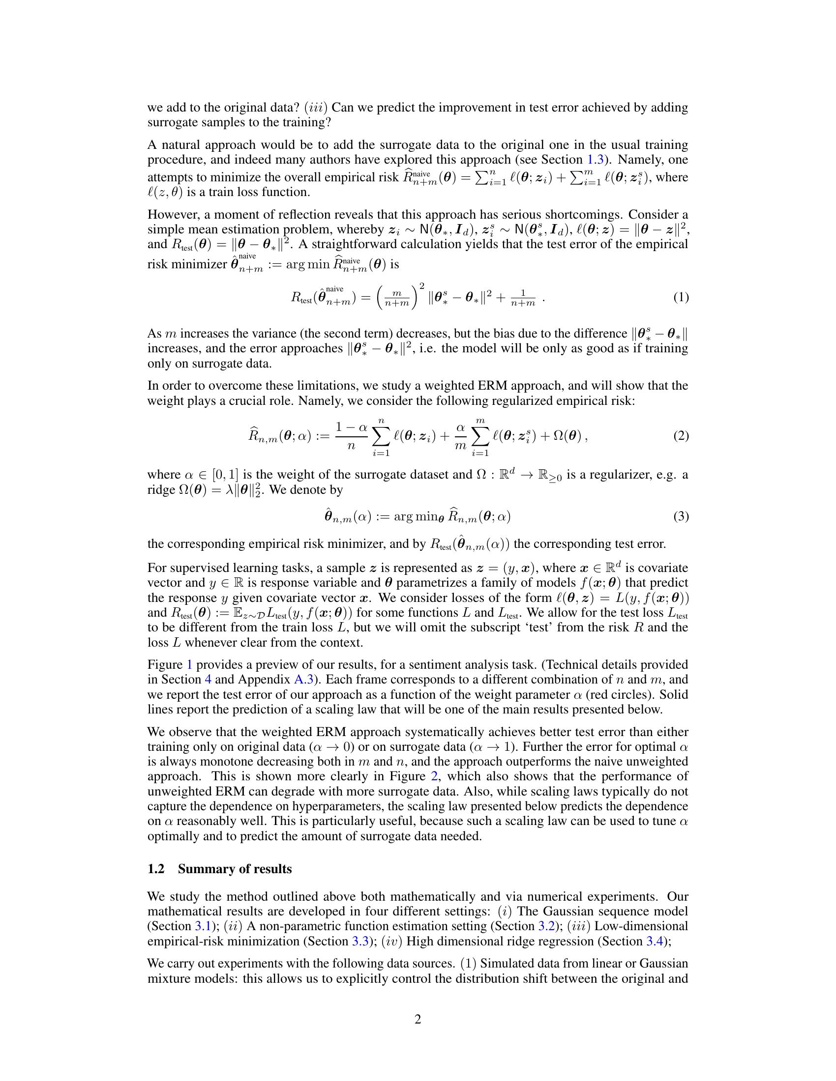
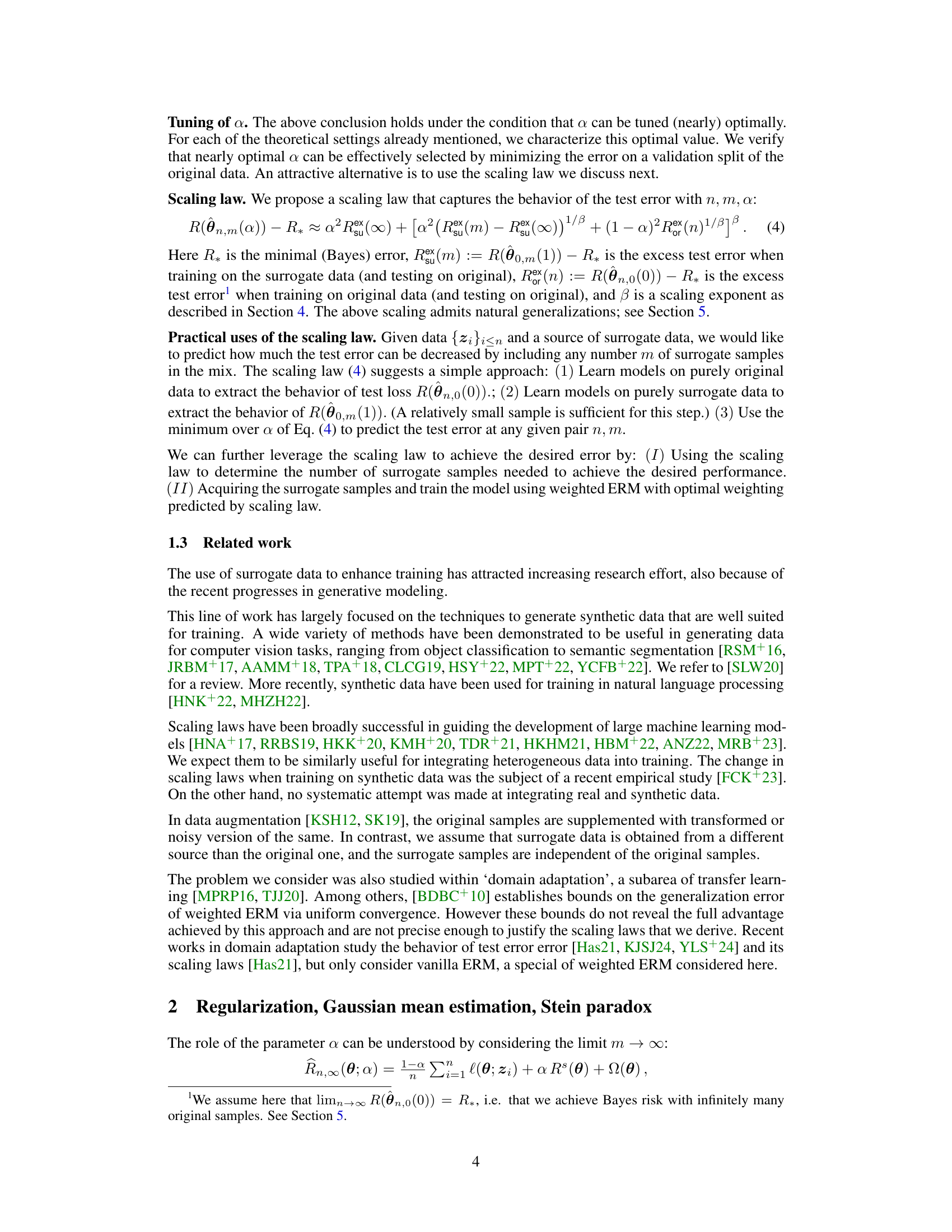
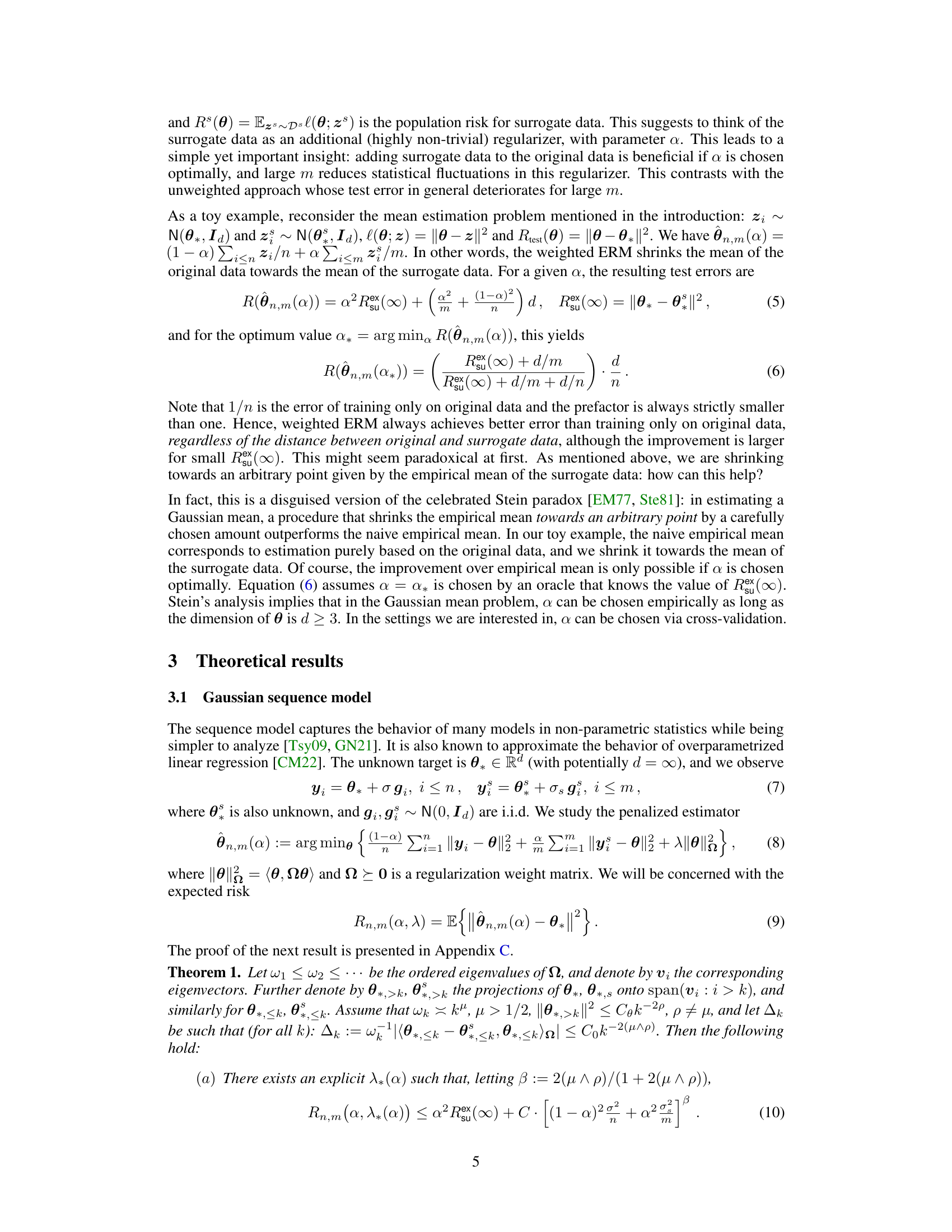
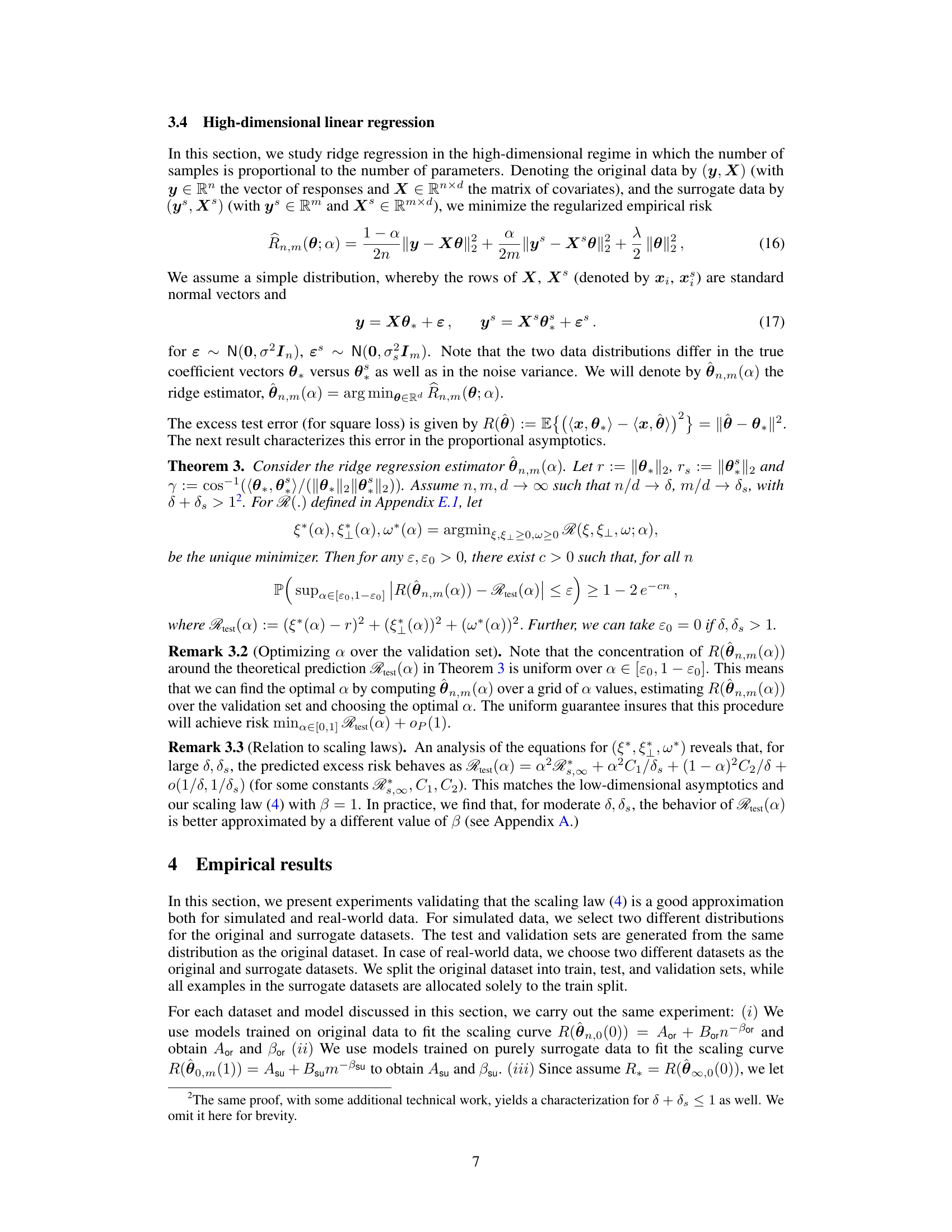
TL;DR#
Many machine learning projects are hampered by the high cost and difficulty of obtaining large amounts of high-quality data. This paper explores using ‘surrogate data’—data from more accessible sources or generated synthetically—to supplement limited real data. The paper investigates the challenges of directly combining real and surrogate data, noting that doing so can lead to suboptimal performance.
The researchers propose a solution: a weighted empirical risk minimization (ERM) method for integrating real and surrogate data. Their mathematical analysis and experiments show that using an optimal weighting scheme significantly improves model accuracy. They further develop a ‘scaling law’ that helps predict the optimal weighting and the amount of surrogate data needed to achieve a target error rate, providing a valuable guideline for practical applications.
Key Takeaways#
Why does it matter?#
This paper is crucial for researchers facing data scarcity in machine learning. It introduces a novel weighted ERM approach, providing a practical and effective way to integrate surrogate data, potentially reducing test error significantly. This opens avenues for cost-effective model training and inspires further research into optimal data integration strategies and scaling laws for mixed-data learning.
Visual Insights#

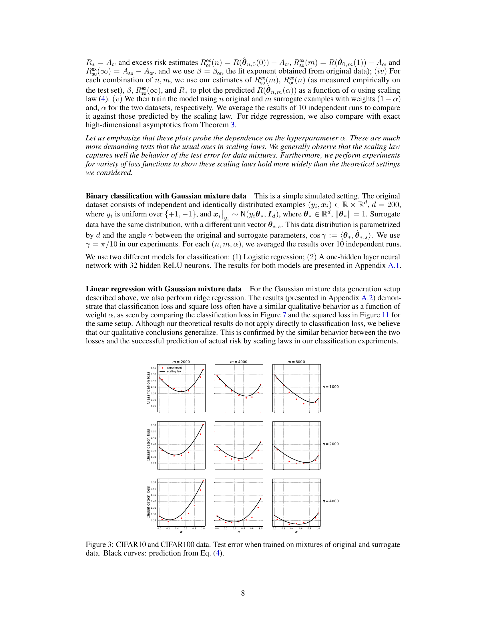
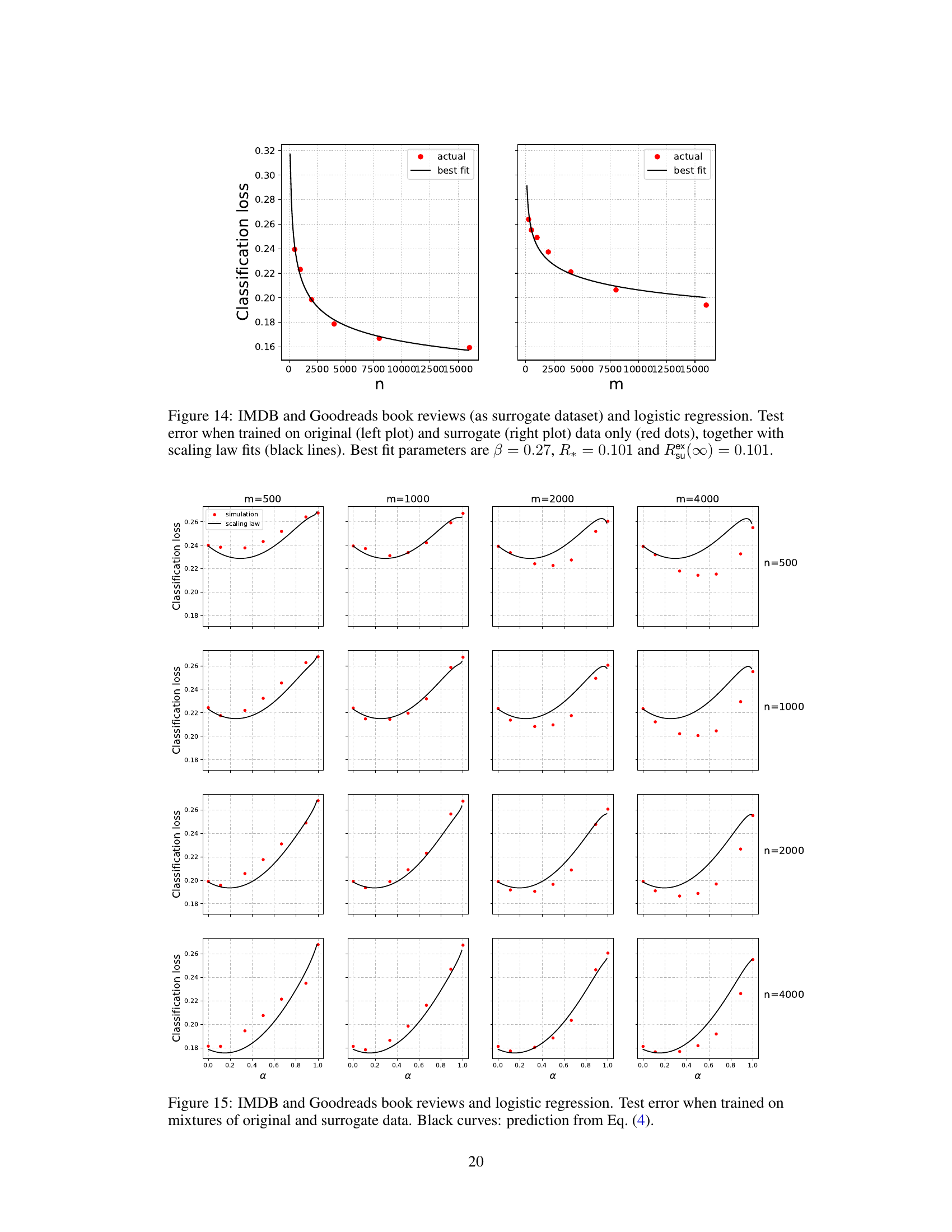
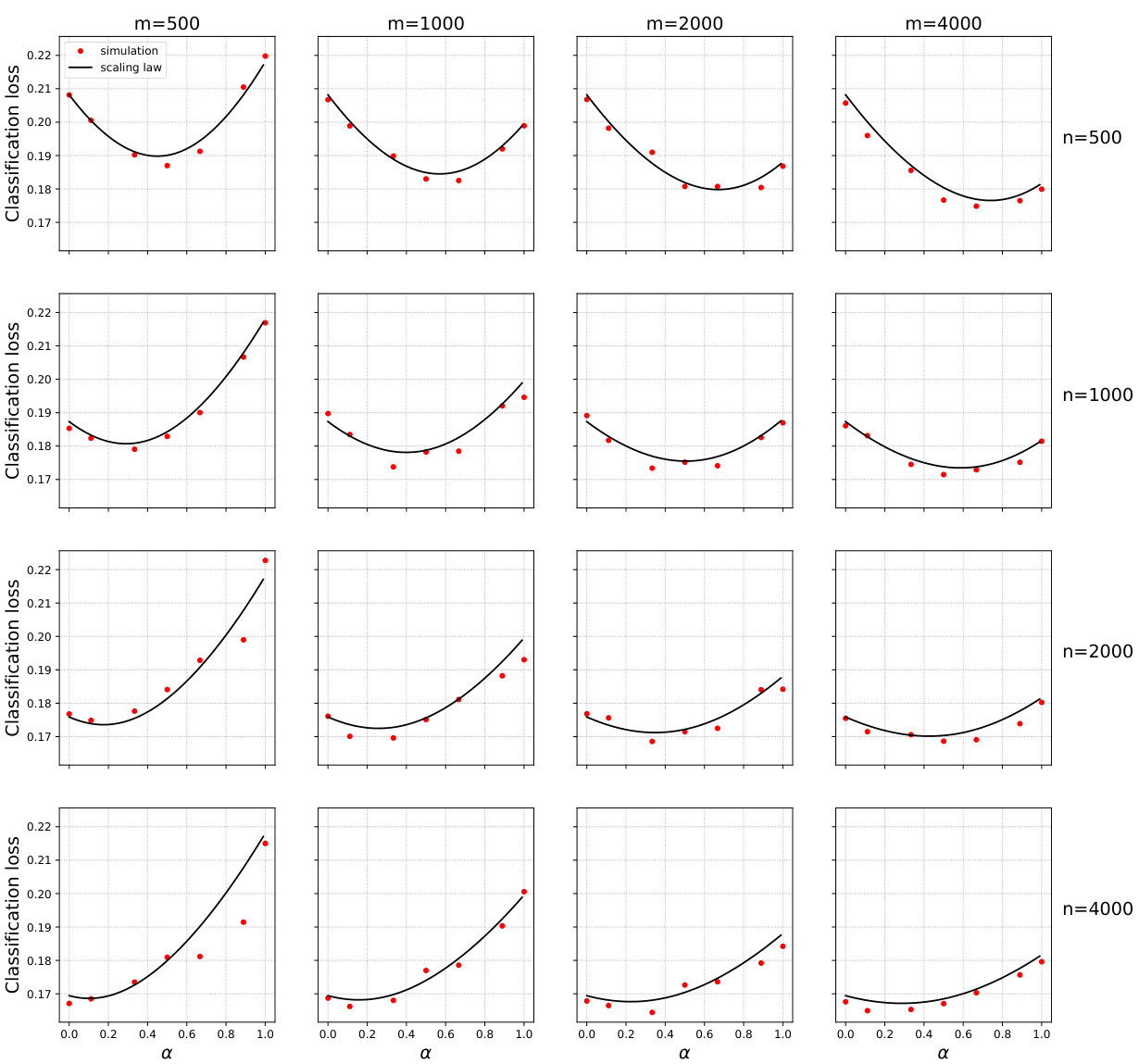
🔼 This figure shows the test error of models trained on mixtures of original and surrogate data for sentiment analysis using IMDB and Rotten Tomatoes datasets. The x-axis represents the weight given to surrogate data (α), ranging from 0 (only original data) to 1 (only surrogate data). The y-axis shows the classification loss. Different curves represent different amounts of original (n) and surrogate (m) data. The black curves represent the prediction based on a scaling law derived in the paper (Equation 4). The figure demonstrates that using a mixture of data with optimal weighting leads to lower test error compared to using only original or surrogate data.
read the caption
Figure 1: IMDB and Rotten Tomatoes data and neural networks. Test error when trained on mixtures of original and surrogate data. Black curves: prediction from Eq. (4).
In-depth insights#
Surrogate Data ERM#
The concept of ‘Surrogate Data ERM’ blends the power of empirical risk minimization (ERM) with the practicality of using readily available, albeit potentially less accurate, data. The core idea is to augment the training process with surrogate data, enhancing model performance by leveraging a larger dataset. While traditional ERM focuses solely on high-quality, target-distribution data, Surrogate Data ERM acknowledges the cost and difficulty associated with acquiring such data. The approach’s effectiveness hinges on appropriately weighting the real and surrogate data points within the ERM framework, preventing the surrogate data from unduly biasing the model. This weighting strategy is crucial; an improper balance could lead to suboptimal or even detrimental effects. Mathematical analysis and empirical experiments are key to determining the optimal weighting schemes. Ultimately, Surrogate Data ERM presents a practical and theoretically grounded solution for situations where high-quality data is scarce or expensive to obtain. A scaling law governing the relationship between the amount of real and surrogate data is a particularly valuable contribution, aiding in predicting model performance and guiding the optimal dataset composition.
Stein’s Paradox Effect#
Stein’s paradox, in the context of this research paper, appears to highlight a surprising phenomenon: incorporating seemingly unrelated surrogate data can improve the accuracy of a model trained on real data. This counterintuitive result arises from the fact that adding surrogate data, even if not directly related to the target distribution, acts as a regularizer, shrinking the model’s parameters towards a more stable and less overfit solution. This effect, akin to Stein’s paradox where shrinking an estimator toward an arbitrary point can improve its accuracy, shows how the model’s bias may be counteracted by the introduction of additional, potentially diverse information that helps generalize better to unseen data. Optimal weighting is crucial; simply mixing real and surrogate data without proper weighting can lead to suboptimal results, potentially even worsening performance. The paper demonstrates the presence of this effect empirically across various models and datasets, suggesting that the phenomenon is robust and not confined to specific experimental settings. This observation suggests new strategies for leveraging readily available, diverse datasets in machine learning.
Scaling Law Insights#
The concept of “Scaling Law Insights” in the context of a machine learning research paper likely refers to the discovery and analysis of predictable relationships between key training parameters (like dataset size, model size, and computational resources) and the resulting model performance. A core insight would be identifying a scaling law that accurately describes the improvement in test error as a function of the amount of real and surrogate data used in training. This would likely involve empirical validation and mathematical analysis of how the relative quantities of real and surrogate data affect model generalization. A strong contribution could be demonstrating a systematic improvement in model performance even when surrogate data is only loosely related to the real data, potentially due to regularization effects. Further analysis could explore how to optimally weight the contributions of real and surrogate data to minimize test error, and whether specific weighting schemes lead to predictable performance gains. The resulting insights would be particularly valuable for guiding practical applications and resource allocation in machine learning projects where high-quality data is scarce or expensive to obtain.
Optimal Weighting Scheme#
The optimal weighting scheme for integrating real and surrogate data in machine learning is a crucial aspect of this research. The core idea revolves around finding the best balance between the information contained in the real data (which is assumed to be of high quality but limited in quantity) and the surrogate data (which is more plentiful but might be lower quality or from a different distribution). Simple averaging of both datasets is shown to be suboptimal, potentially leading to increased test error as the quantity of surrogate data increases. Instead, a weighted empirical risk minimization (ERM) approach is proposed, where a weight parameter, α, controls the contribution of each data source to the training process. Determining the optimal value of α is key to minimizing the test error. The paper investigates this problem mathematically and empirically, demonstrating that finding this optimal weight is important, and that simply adding surrogate data without optimal weighting does not guarantee improved performance. Moreover, the paper introduces a scaling law to approximately predict the optimal weighting scheme, allowing for efficient estimation of the best α and an understanding of how the amount of surrogate data influences the model’s accuracy.
Future Research#
Future research directions stemming from this work could explore refined scaling laws, potentially incorporating model architecture and hyperparameter settings for more precise predictions of optimal surrogate data allocation. Investigating the theoretical underpinnings across diverse model classes beyond the ones studied, such as deep networks, is crucial. A focus on understanding the impact of distribution shifts between real and surrogate data warrants attention, exploring different metrics and developing methods for quantifying and mitigating negative effects. Developing efficient algorithms to identify optimal surrogate data selection strategies, possibly using meta-learning or reinforcement learning approaches, holds promise. Finally, examining the broader implications, particularly concerning fairness and bias in machine learning, in the context of surrogate data integration is essential for responsible AI development.
More visual insights#
More on figures

🔼 This figure compares the performance of unweighted and optimally weighted empirical risk minimization (ERM) approaches. The x-axis represents the amount of surrogate data (m), and the y-axis shows the classification loss. The plot reveals that the optimally weighted ERM consistently outperforms the unweighted approach, achieving lower classification loss across different amounts of surrogate data. This highlights the importance of optimal weighting when integrating surrogate data into model training.
read the caption
Figure 2: Performance of unweighted vs weighted ERM approach for the setting in Figure 1

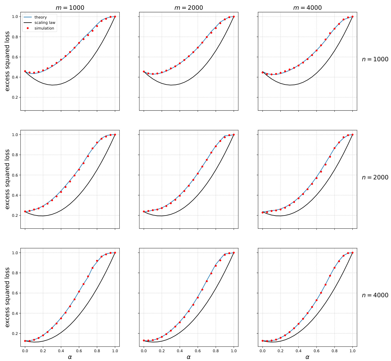
🔼 This figure shows the test error of models trained on mixtures of original and surrogate data for different combinations of the number of original samples (n) and surrogate samples (m). The x-axis represents the weight parameter α, which controls the contribution of surrogate data in the training process. The red dots represent the empirical test error obtained from experiments, while the black curves show the predictions of a scaling law (Equation 4 from the paper). The figure demonstrates that integrating surrogate data can significantly reduce the test error, even when the surrogate data is different from the original data. The optimal weight α is neither 0 nor 1 (i.e. training only on original or only on surrogate data), suggesting the importance of optimally weighing the contribution of both datasets.
read the caption
Figure 1: IMDB and Rotten Tomatoes data and neural networks. Test error when trained on mixtures of original and surrogate data. Black curves: prediction from Eq. (4).
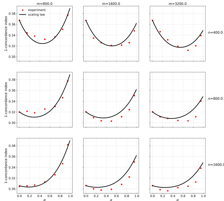
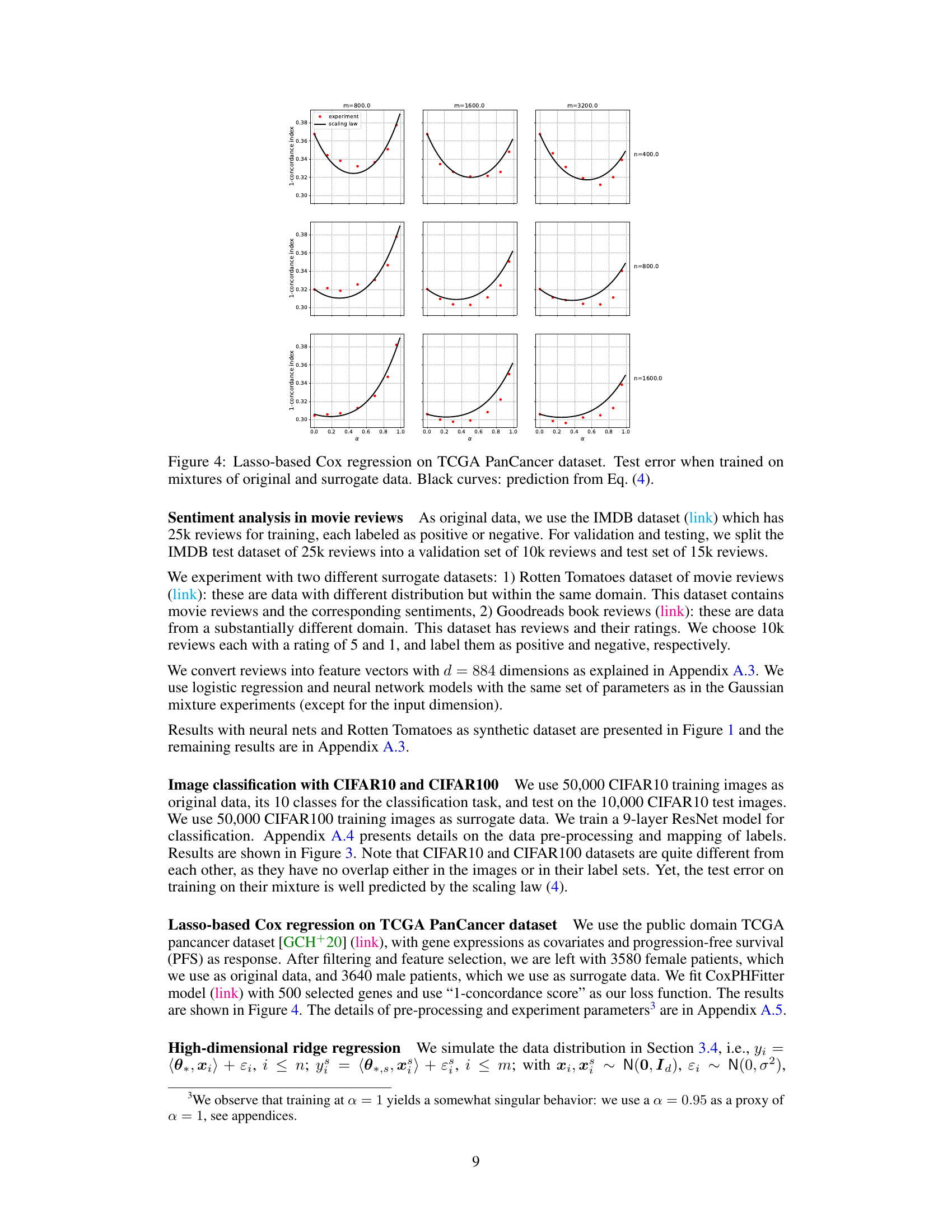
🔼 This figure shows the test error of Lasso-based Cox regression on the TCGA PanCancer dataset when trained on mixtures of original and surrogate data. The x-axis represents the weight parameter (alpha) given to the surrogate data, ranging from 0 to 1. Different panels show the results for different combinations of the number of original data points (n) and the number of surrogate data points (m). The red dots represent the experimentally observed test error, while the black curves represent the test error predicted by equation (4), a scaling law derived in the paper. The scaling law aims to capture how the test error changes as a function of alpha, n, and m.
read the caption
Figure 4: Lasso-based Cox regression on TCGA PanCancer dataset. Test error when trained on mixtures of original and surrogate data. Black curves: prediction from Eq. (4).
🔼 This figure shows the test error achieved when training neural networks on mixtures of original and surrogate data. The x-axis represents the weight parameter (α) given to the surrogate data in the training process, varying from 0 (only original data) to 1 (only surrogate data). The y-axis shows the classification loss. Different curves represent different combinations of the number of original data points (n) and the number of surrogate data points (m). The black curves represent the prediction from Equation 4 (a scaling law derived in the paper) and closely follow the experimental results.
read the caption
Figure 1: IMDB and Rotten Tomatoes data and neural networks. Test error when trained on mixtures of original and surrogate data. Black curves: prediction from Eq. (4).
🔼 This figure displays the test error achieved when training neural networks on mixtures of original and surrogate data. The x-axis represents the weight parameter α, which controls the weighting between original and surrogate data. Different points represent different dataset sizes (n for original, m for surrogate). Red dots represent the actual test error obtained through experiments. The black curves represent the predictions generated by Equation 4, which is a scaling law proposed by the paper to model the relationship between dataset size, weight parameter, and test error.
read the caption
Figure 1: IMDB and Rotten Tomatoes data and neural networks. Test error when trained on mixtures of original and surrogate data. Black curves: prediction from Eq. (4).

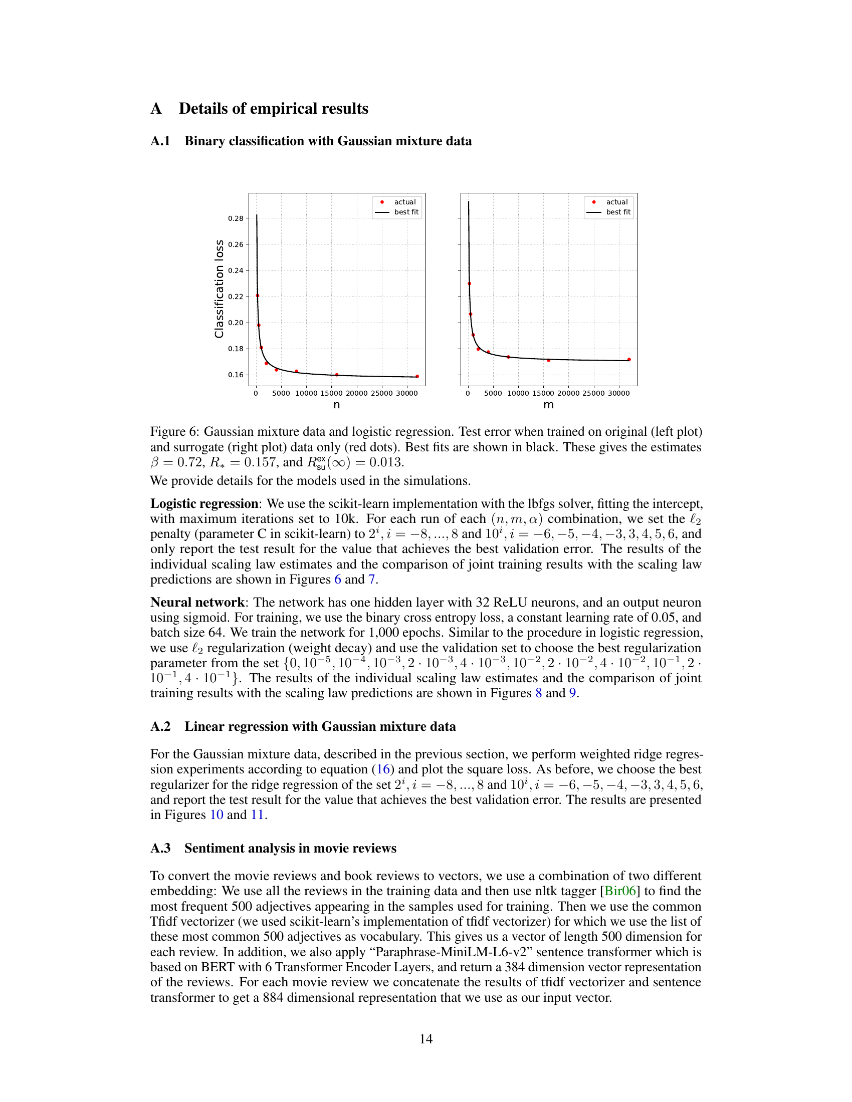
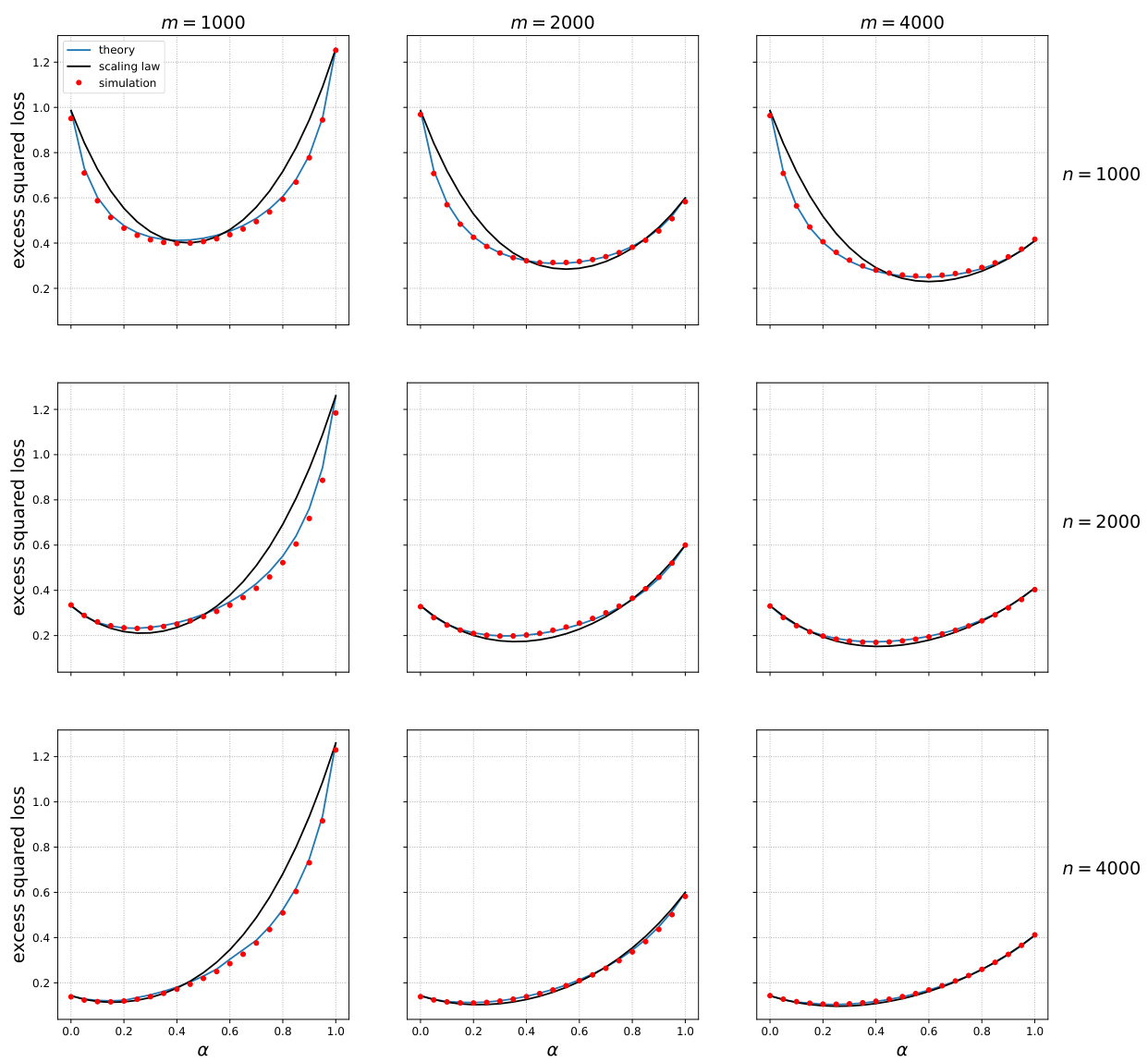
🔼 This figure displays the results of an experiment on Gaussian mixture data using logistic regression. It shows the test error achieved when training models on mixtures of real data (n samples) and surrogate data (m samples), for various values of the mixing parameter (alpha, α). The x-axis represents alpha (0 to 1), indicating the proportion of surrogate data used in training. The y-axis represents the classification loss. Different rows correspond to varying amounts of real data (n), while different columns correspond to varying amounts of surrogate data (m). The black curves represent the prediction from the scaling law (4), which is a mathematical model the authors developed to approximate the test error as a function of n, m, and α. This scaling law is a core finding of the paper, showing the relationship between the quantity of real and surrogate data and the resulting model performance.
read the caption
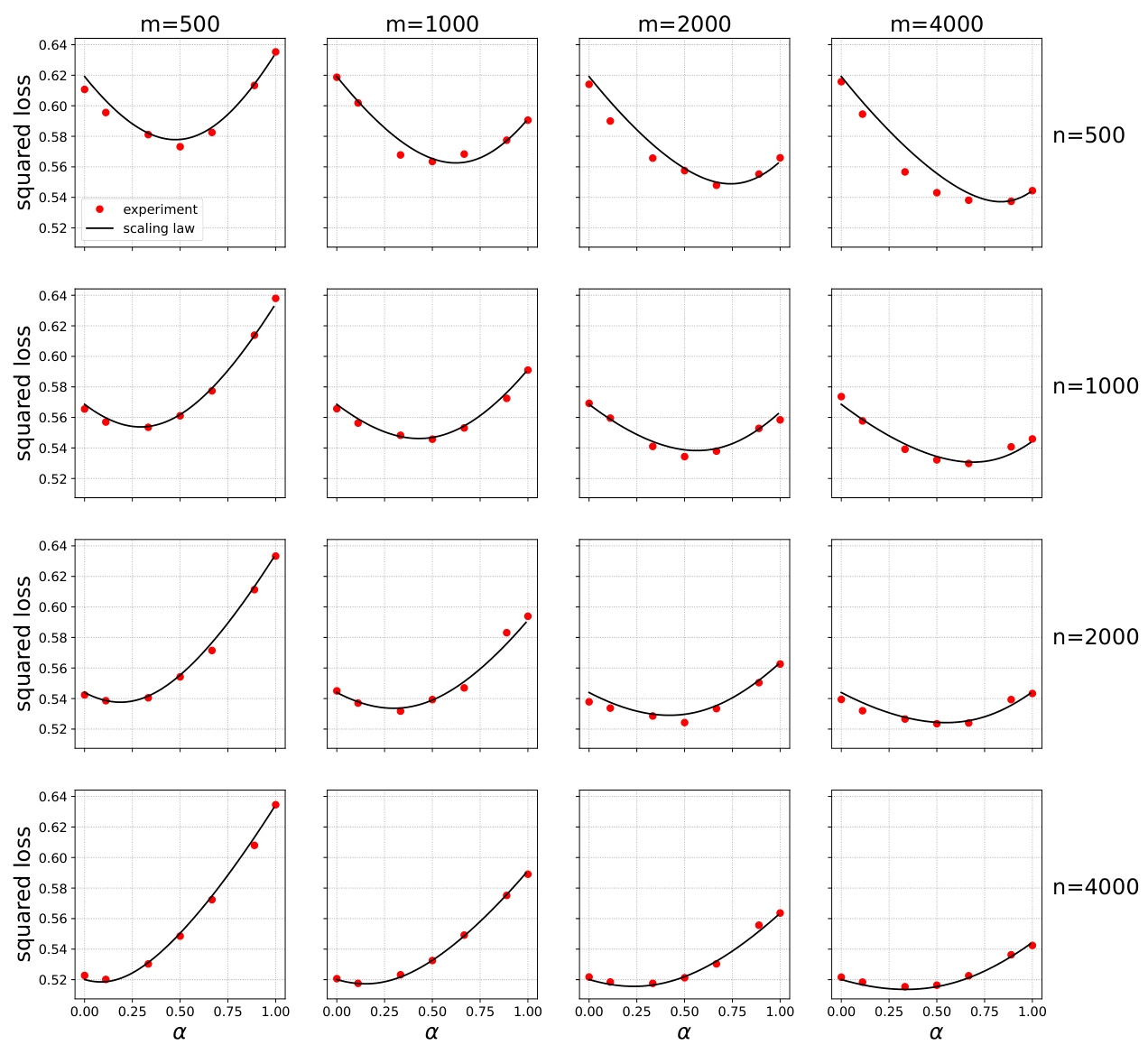
Figure 7: Gaussian mixture data and logistic regression. Test error when trained on mixtures of original (n varying by row) and surrogate (m varying by column) data. Black curves: scaling formula (4).
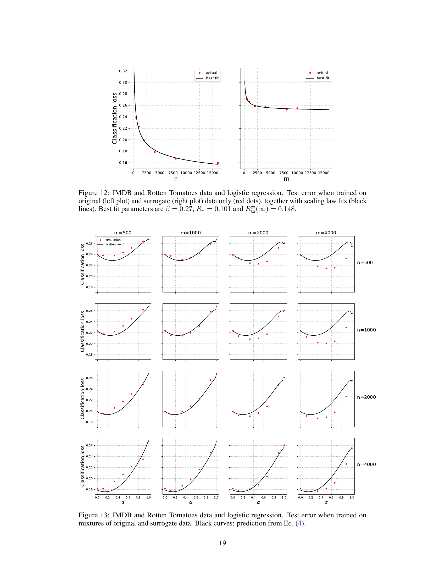
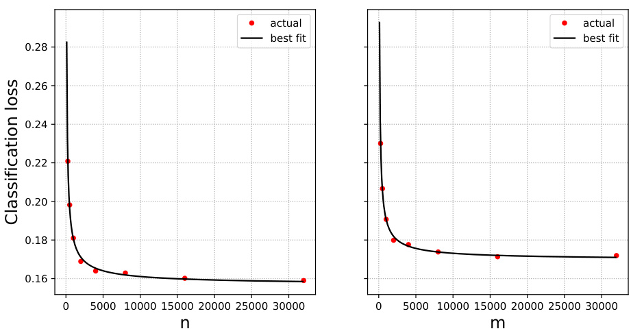
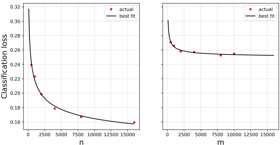
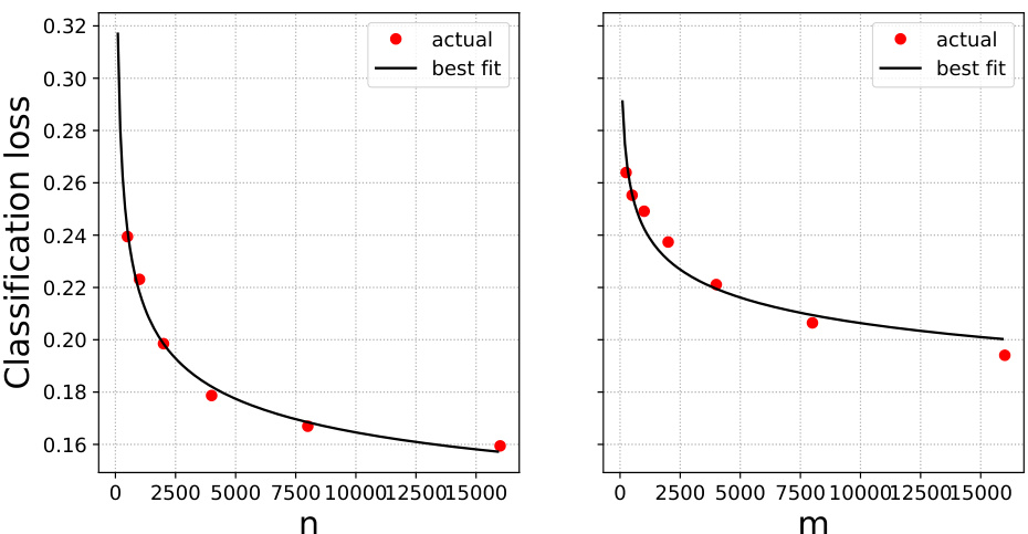
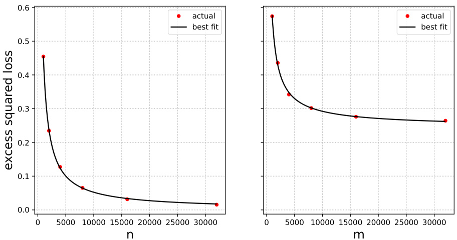
🔼 The figure shows the test error for IMDB movie reviews (original data) and Rotten Tomatoes movie reviews (surrogate data) using logistic regression. The left plot shows the test error when trained only on the original data, and the right plot shows the test error when trained only on the surrogate data. The black lines are the best fits of the scaling law, which has parameters β = 0.27, R* = 0.101, and R(∞) = 0.148.
read the caption
Figure 12: IMDB and Rotten Tomatoes data and logistic regression. Test error when trained on original (left plot) and surrogate (right plot) data only (red dots), together with scaling law fits (black lines). Best fit parameters are β = 0.27, R* = 0.101 and R(∞) = 0.148.
🔼 This figure visualizes the test error achieved when training neural networks on mixtures of real and surrogate data from IMDB and Rotten Tomatoes datasets. The test error is plotted as a function of the weight parameter α, which controls the contribution of surrogate data. Each subplot represents a different combination of the number of original (n) and surrogate (m) data points. The black curves represent a scaling law prediction (Eq. 4 from the paper) which aims to model the relationship between the test error and these parameters.
read the caption
Figure 1: IMDB and Rotten Tomatoes data and neural networks. Test error when trained on mixtures of original and surrogate data. Black curves: prediction from Eq. (4).
🔼 This figure displays the test error achieved when training neural networks on mixtures of real and surrogate data from the IMDB and Rotten Tomatoes datasets. The x-axis represents the weighting parameter (alpha) used to balance the contribution of real and surrogate data, with 0 representing only real data and 1 representing only surrogate data. The y-axis shows the classification loss (test error). Different plots show the effect of varying the number of original (n) and surrogate (m) samples. The black curves represent the prediction of a scaling law derived in the paper (Eq. (4)), demonstrating how well the law approximates the actual results. The figure highlights the potential benefits of using surrogate data to improve model performance.
read the caption
Figure 1: IMDB and Rotten Tomatoes data and neural networks. Test error when trained on mixtures of original and surrogate data. Black curves: prediction from Eq. (4).
🔼 This figure shows the test error when training a neural network model on mixtures of original and surrogate data for sentiment analysis. The x-axis represents the weight parameter (alpha) given to the surrogate data in the weighted ERM approach. The y-axis shows the test error. Different colored dots represent different combinations of the number of original data points (n) and surrogate data points (m). The black curves show predictions based on the scaling law derived in the paper (Equation 4). The figure demonstrates the impact of both the weight parameter and the amount of surrogate data on model performance.
read the caption
Figure 1: IMDB and Rotten Tomatoes data and neural networks. Test error when trained on mixtures of original and surrogate data. Black curves: prediction from Eq. (4).
🔼 This figure shows the test error achieved by training neural networks on mixtures of real and surrogate data. The x-axis represents the weight given to the surrogate data (α), ranging from 0 (only real data) to 1 (only surrogate data). Each curve represents a different combination of the number of real (n) and surrogate (m) data points. The red dots indicate the observed test error, while the black curves show the predictions made by the scaling law (equation 4) derived in the paper. The scaling law attempts to predict the test error as a function of α, n, and m.
read the caption
Figure 1: IMDB and Rotten Tomatoes data and neural networks. Test error when trained on mixtures of original and surrogate data. Black curves: prediction from Eq. (4).
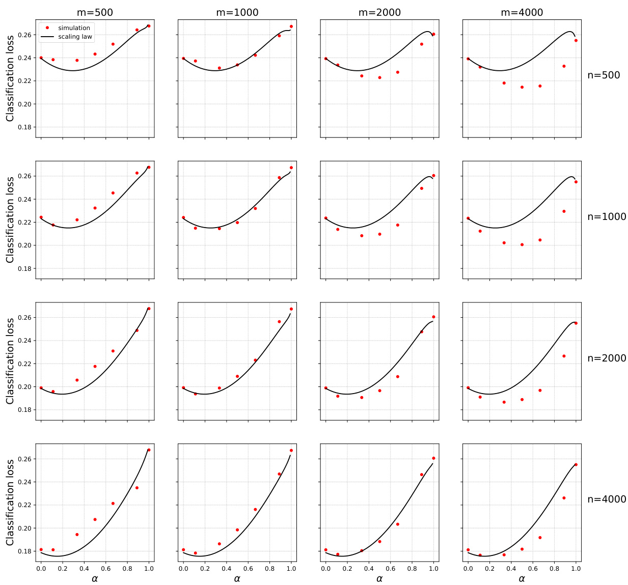
🔼 This figure displays the test error results from training neural networks on mixtures of original and surrogate data. The x-axis represents the weight assigned to the surrogate data (alpha), ranging from 0 (only original data) to 1 (only surrogate data). The y-axis shows the classification loss (test error). Different plots represent varying numbers of original (n) and surrogate (m) data points. The black curves are predictions based on Equation (4) from the paper, which is a scaling law that relates test error to n, m, and alpha.
read the caption
Figure 1: IMDB and Rotten Tomatoes data and neural networks. Test error when trained on mixtures of original and surrogate data. Black curves: prediction from Eq. (4).
🔼 This figure shows the test error achieved by training neural networks on mixtures of original and surrogate data, for various ratios of original to surrogate data (represented by the weighting parameter α). The plot displays the results for different numbers of original (n) and surrogate (m) samples. The black curves represent the predictions of a scaling law (Equation 4 from the paper) which the authors propose to approximate the test error. The comparison of the actual test error (red dots) to the scaling law’s prediction illustrates the accuracy of the proposed scaling law in predicting test error based on the amount of original and surrogate data used in training.
read the caption
Figure 1: IMDB and Rotten Tomatoes data and neural networks. Test error when trained on mixtures of original and surrogate data. Black curves: prediction from Eq. (4).

🔼 This figure shows the test error of models trained on mixtures of original and surrogate data for sentiment analysis using IMDB and Rotten Tomatoes reviews. The x-axis represents the weight parameter α, which balances the contribution of original and surrogate data. Different subplots show the results for varying numbers (n and m) of original and surrogate data points, respectively. The red dots represent the empirical test error obtained through experiments. The black curves show the prediction of a scaling law (Equation 4 from the paper) that approximates the relationship between the test error, the weight parameter α, and the number of data points.
read the caption
Figure 1: IMDB and Rotten Tomatoes data and neural networks. Test error when trained on mixtures of original and surrogate data. Black curves: prediction from Eq. (4).
🔼 This figure shows the test error for logistic regression models trained on IMDB movie review data (original data) and Rotten Tomatoes movie review data (surrogate data) separately. The left plot shows the performance of models trained only on varying amounts of original data (IMDB), while the right plot shows performance on surrogate data (Rotten Tomatoes). The red dots represent the actual test error for different sample sizes. The black lines show the best fit to the data using a scaling law, with parameters β, R*, and Rex(∞) estimated to be 0.27, 0.101, and 0.148, respectively. This figure illustrates the behavior of the test error when only one data source is used in the training of the model.
read the caption
Figure 12: IMDB and Rotten Tomatoes data and logistic regression. Test error when trained on original (left plot) and surrogate (right plot) data only (red dots), together with scaling law fits (black lines). Best fit parameters are β = 0.27, R* = 0.101 and Rex(∞) = 0.148.
🔼 This figure shows the test error for sentiment analysis using neural networks trained on mixtures of original and surrogate data. The x-axis represents the weight parameter (α) given to surrogate data in the weighted ERM approach, ranging from 0 (only original data) to 1 (only surrogate data). Different panels show the results for varying amounts of original (n) and surrogate (m) data. The red dots represent the experimental results, and the black curves show the predictions from a scaling law (Equation 4 in the paper) that attempts to model the relationship between test error, α, n, and m.
read the caption
Figure 1: IMDB and Rotten Tomatoes data and neural networks. Test error when trained on mixtures of original and surrogate data. Black curves: prediction from Eq. (4).

🔼 This figure compares the performance of unweighted and optimally weighted empirical risk minimization (ERM) methods. The x-axis represents the number of surrogate samples (m), and the y-axis shows the test error. The plot demonstrates that the weighted ERM approach consistently outperforms the unweighted approach, highlighting the importance of optimal weighting when integrating surrogate data into training.
read the caption
Figure 2: Performance of unweighted vs weighted ERM approach for the setting in Figure 1
🔼 This figure shows the test error when training a neural network model on mixtures of original and surrogate data for sentiment analysis using IMDB and Rotten Tomatoes datasets. The x-axis represents the weight parameter (α) of the surrogate data, and the y-axis represents the test error. The red dots represent the actual test error obtained experimentally, while the black curves represent the predicted test error based on equation (4) from the paper. The figure demonstrates how the optimal weighting scheme significantly reduces test error compared to using only original or only surrogate data.
read the caption
Figure 1: IMDB and Rotten Tomatoes data and neural networks. Test error when trained on mixtures of original and surrogate data. Black curves: prediction from Eq. (4).

🔼 This figure shows the test error when training a neural network on mixtures of original and surrogate data for sentiment analysis. The x-axis represents the weight given to the surrogate data (alpha), and the y-axis shows the classification loss. Different panels show various sizes of the original (n) and surrogate (m) datasets. The black curves represent the predictions of a scaling law (equation 4 from the paper) which is a model for how the test error depends on the amount of original and surrogate data.
read the caption
Figure 1: IMDB and Rotten Tomatoes data and neural networks. Test error when trained on mixtures of original and surrogate data. Black curves: prediction from Eq. (4).

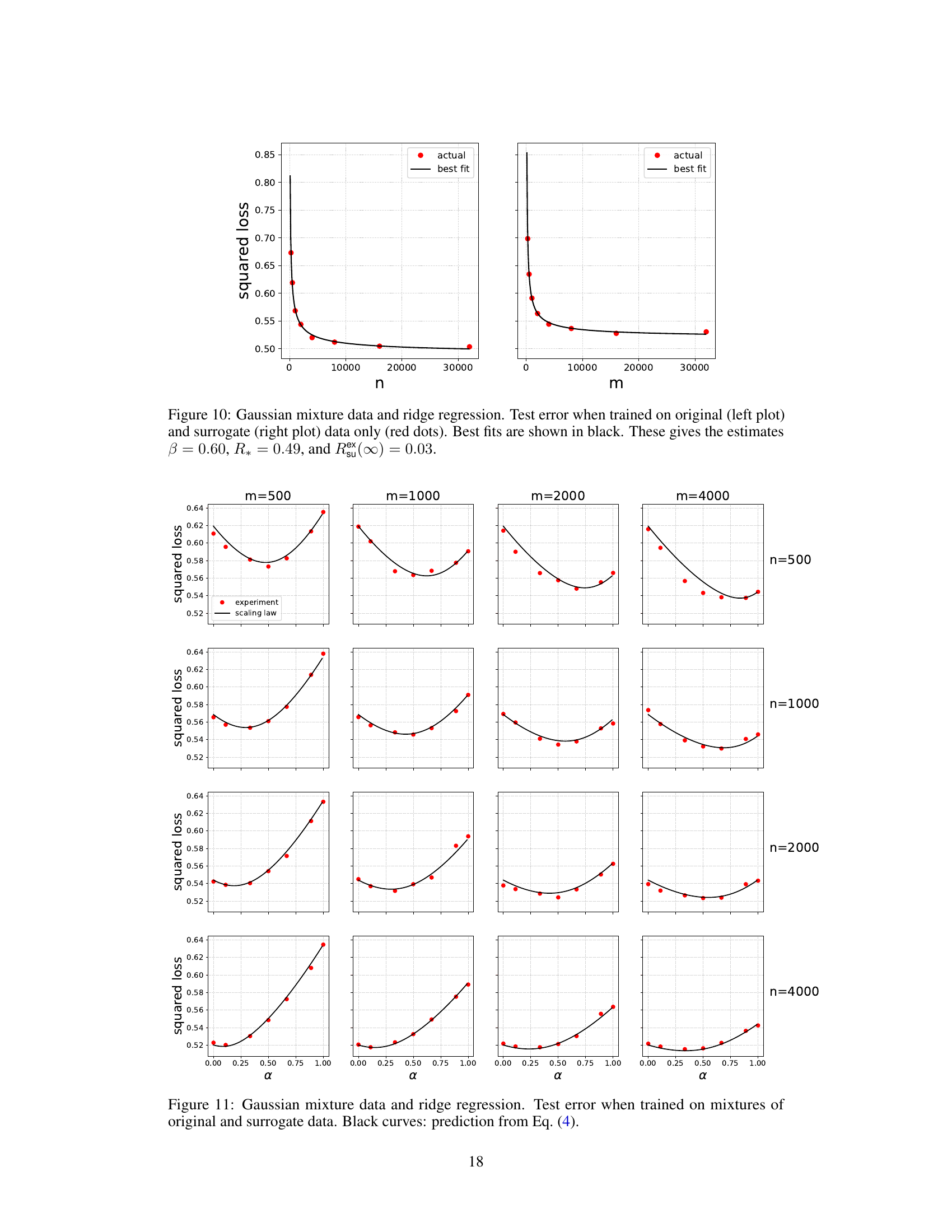
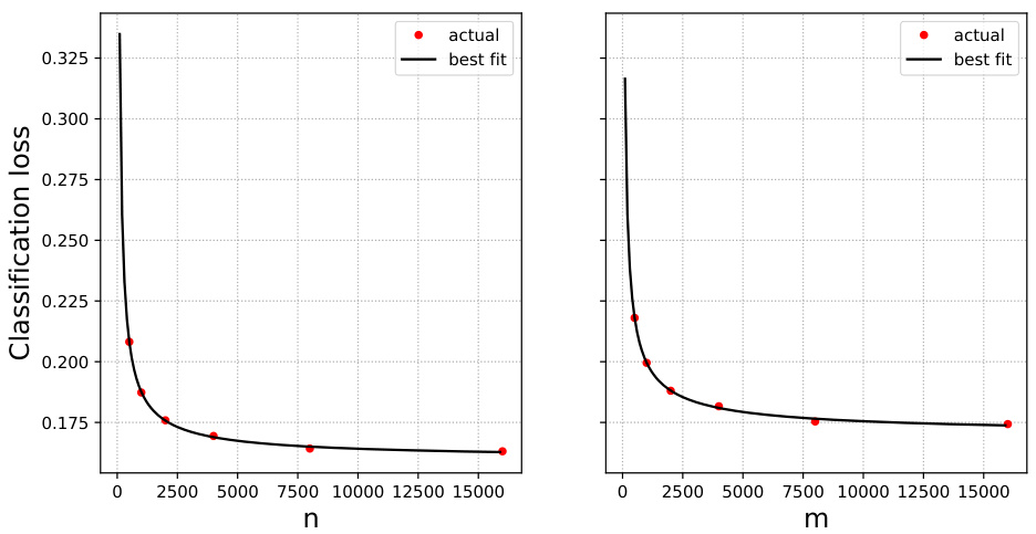
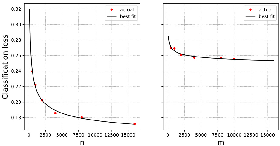
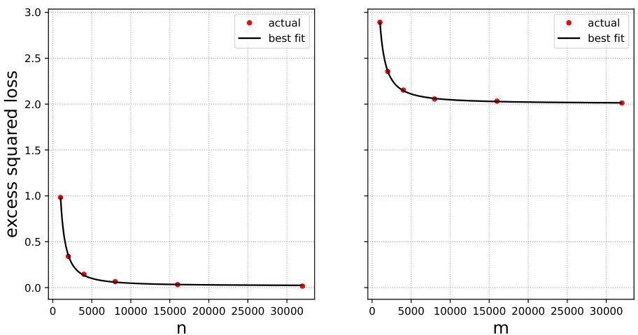
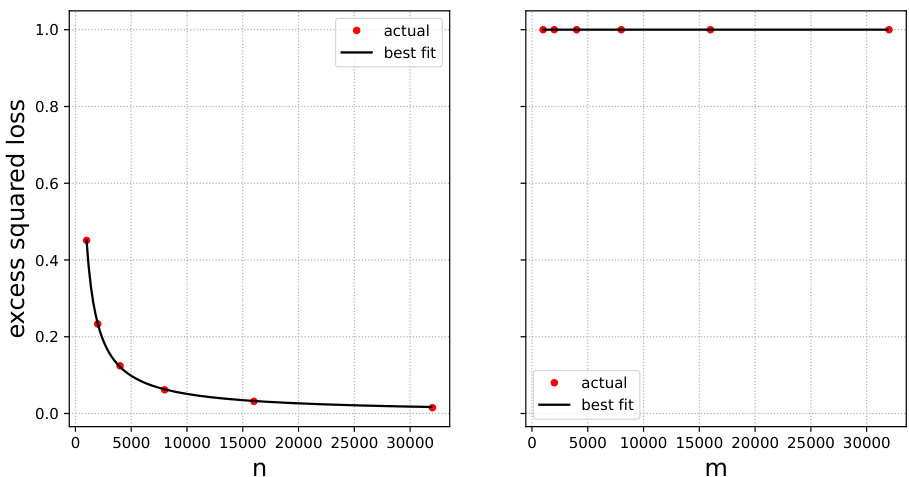
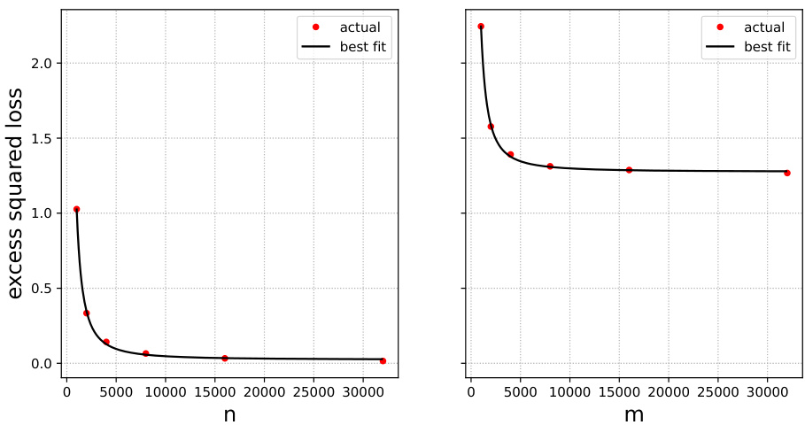
🔼 This figure shows the test error results when training a ridge regression model using only original data (left) and only surrogate data (right). The red dots represent the actual test errors obtained from experiments, while the black curves represent the best-fit curves based on the scaling law. This illustrates the test error behaviour of the model under different sample sizes and the data source.
read the caption
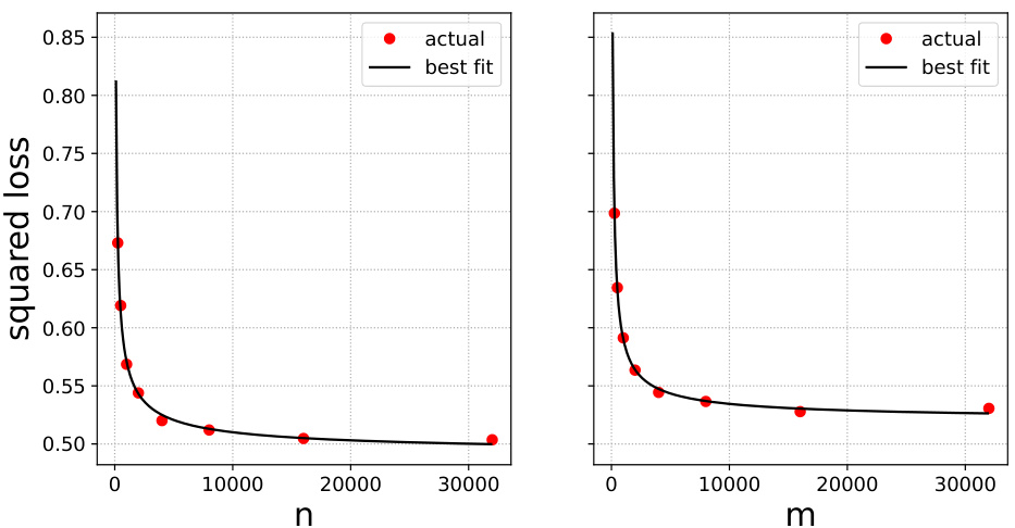
Figure 10: Gaussian mixture data and ridge regression. Test error when trained on original (left plot) and surrogate (right plot) data only (red dots). Best fits are shown in black. These gives the estimates β = 0.60, R* = 0.49, and Rex(∞) = 0.03.
🔼 This figure shows the test error when training neural networks on mixtures of original and surrogate data. It demonstrates that using a weighted combination of both datasets (optimal α) generally leads to lower error than using either dataset alone. The black curves represent predictions from a derived scaling law (Eq. 4) which approximates the relationship between test error, the amount of original and surrogate data, and the weighting scheme.
read the caption
Figure 1: IMDB and Rotten Tomatoes data and neural networks. Test error when trained on mixtures of original and surrogate data. Black curves: prediction from Eq. (4).

🔼 This figure shows the test error of ridge regression models trained only on original data (left) and surrogate data (right). The red dots represent the actual test error obtained from the experiments. The black lines represent the best fit curves. The parameters β, R*, and Rex(∞) are estimated from the best fit curves.
read the caption
Figure 10: Gaussian mixture data and ridge regression. Test error when trained on original (left plot) and surrogate (right plot) data only (red dots). Best fits are shown in black. These gives the estimates β = 0.60, R* = 0.49, and Rex(∞) = 0.03.

🔼 This figure shows the test error of models trained on mixtures of original and surrogate data for sentiment analysis. The x-axis represents the weight parameter (α) of the surrogate data, ranging from 0 (only original data) to 1 (only surrogate data). The y-axis shows the classification loss (test error). The plots demonstrate the performance for different combinations of original (n) and surrogate (m) data points. The black curves represent the prediction of the scaling law described by Equation (4) in the paper, showing a good match with the experimental results (red dots). The figure highlights that optimally weighting the combined data sources leads to lower test error compared to using only original or surrogate data.
read the caption
Figure 1: IMDB and Rotten Tomatoes data and neural networks. Test error when trained on mixtures of original and surrogate data. Black curves: prediction from Eq. (4).
🔼 This figure displays the test error for ridge regression on Gaussian mixture data when trained using only original data (left) and only surrogate data (right). Red dots show the actual test error for different sample sizes. The black lines represent the best fit curves obtained, providing estimates for the scaling exponent (β), minimal error (R*), and excess test error with infinite surrogate data (Rex(∞)). These parameters offer insights into the behavior of the model’s performance.
read the caption
Figure 10: Gaussian mixture data and ridge regression. Test error when trained on original (left plot) and surrogate (right plot) data only (red dots). Best fits are shown in black. These gives the estimates β = 0.60, R* = 0.49, and Rex(∞) = 0.03.

🔼 This figure shows the test error of sentiment analysis models trained on mixtures of original and surrogate data for various ratios (α) of surrogate data. The x-axis represents the weight (α) given to the surrogate data, ranging from 0 (only original data) to 1 (only surrogate data). The y-axis represents the classification loss. Each subplot shows results for different sizes of original (n) and surrogate (m) datasets. The black curves represent the predictions from a scaling law presented in the paper (Equation 4), illustrating how well the scaling law can capture the relationship between test error, data size, and the mixture ratio.
read the caption
Figure 1: IMDB and Rotten Tomatoes data and neural networks. Test error when trained on mixtures of original and surrogate data. Black curves: prediction from Eq. (4).
🔼 This figure shows the test error of sentiment analysis models trained on mixtures of original and surrogate data. The x-axis represents the weight parameter (α) given to the surrogate data in a weighted empirical risk minimization (ERM) approach. The different curves correspond to different numbers of original (n) and surrogate (m) data points. The red circles represent the experimental results, while the black curves are predictions based on a scaling law (Eq. 4) described in the paper. The plot demonstrates that combining original and surrogate data, with optimal weighting, reduces test error.
read the caption
Figure 1: IMDB and Rotten Tomatoes data and neural networks. Test error when trained on mixtures of original and surrogate data. Black curves: prediction from Eq. (4).
🔼 This figure shows the test error of models trained on mixtures of original and surrogate data for different combinations of the number of original data points (n) and surrogate data points (m). The x-axis represents the weight (α) given to the surrogate data in the weighted empirical risk minimization (ERM) approach. The red dots represent the actual test error obtained from the experiments, while the black curves show the test error predicted by the scaling law (Equation 4) presented in the paper. The figure demonstrates that incorporating surrogate data, even with optimal weighting, can significantly reduce the test error.
read the caption
Figure 1: IMDB and Rotten Tomatoes data and neural networks. Test error when trained on mixtures of original and surrogate data. Black curves: prediction from Eq. (4).
🔼 This figure shows the test error when training only on original data (left) and only on surrogate data (right). The red dots represent the actual test errors, while the black lines represent the best fit using the scaling law. The parameters of the best fit are also provided. This helps to illustrate the behavior of the test error for different amounts of original and surrogate data, highlighting the impact of the surrogate data on the test error.
read the caption
Figure 10: Gaussian mixture data and ridge regression. Test error when trained on original (left plot) and surrogate (right plot) data only (red dots). Best fits are shown in black. These gives the estimates β = 0.60, R* = 0.49, and Rex(∞) = 0.03.

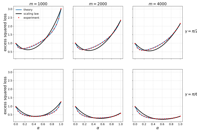
🔼 This figure shows the results of ridge regression experiments on simulated data. The experiments vary the number of surrogate samples (m) and the angle γ between the original and surrogate parameters. The plot shows the excess squared loss as a function of the weight parameter α. The top row shows results where the original and surrogate data are orthogonal (γ = π/2), while the bottom row shows results where they are closer (γ = π/6). The figure demonstrates how the optimal weight parameter α and test error changes as a function of the number of samples.
read the caption
Figure 5: Ridge regression on simulated data. Here d = 500, n = 1000, σ² = σ² = 1, ||0*|| = ||0*,s|| = 1, regul. par. λ = 2-10, and m varies by column. Top row γ = π/2, bottom row γ = π/6.
Full paper#

