TL;DR#
Large-scale visual datasets, crucial for training AI models, are often biased, leading to unfair and inaccurate models. Previous studies demonstrated that these datasets can be easily classified by AI models, indicating inherent biases. However, the exact nature of these biases remained unclear, making it difficult to address the problem effectively.
This paper introduces a comprehensive framework to identify and analyze biases in visual datasets. The researchers employed various image transformations to isolate different visual attributes (semantic, structural, color, etc.) and assessed their contribution to dataset classification accuracy. They further used object-level queries and natural language processing to gain detailed insights into the semantic characteristics of each dataset. The findings reveal the concrete forms of bias and provide actionable insights for creating more diverse and representative datasets.
Key Takeaways#
Why does it matter?#
This paper is crucial for AI researchers because it directly addresses the critical issue of bias in large-scale visual datasets, a problem hindering the development of fair and generalizable AI models. The framework presented offers a novel approach to identifying and understanding bias, thereby guiding the creation of more inclusive and representative datasets, essential for advancing the field.
Visual Insights#

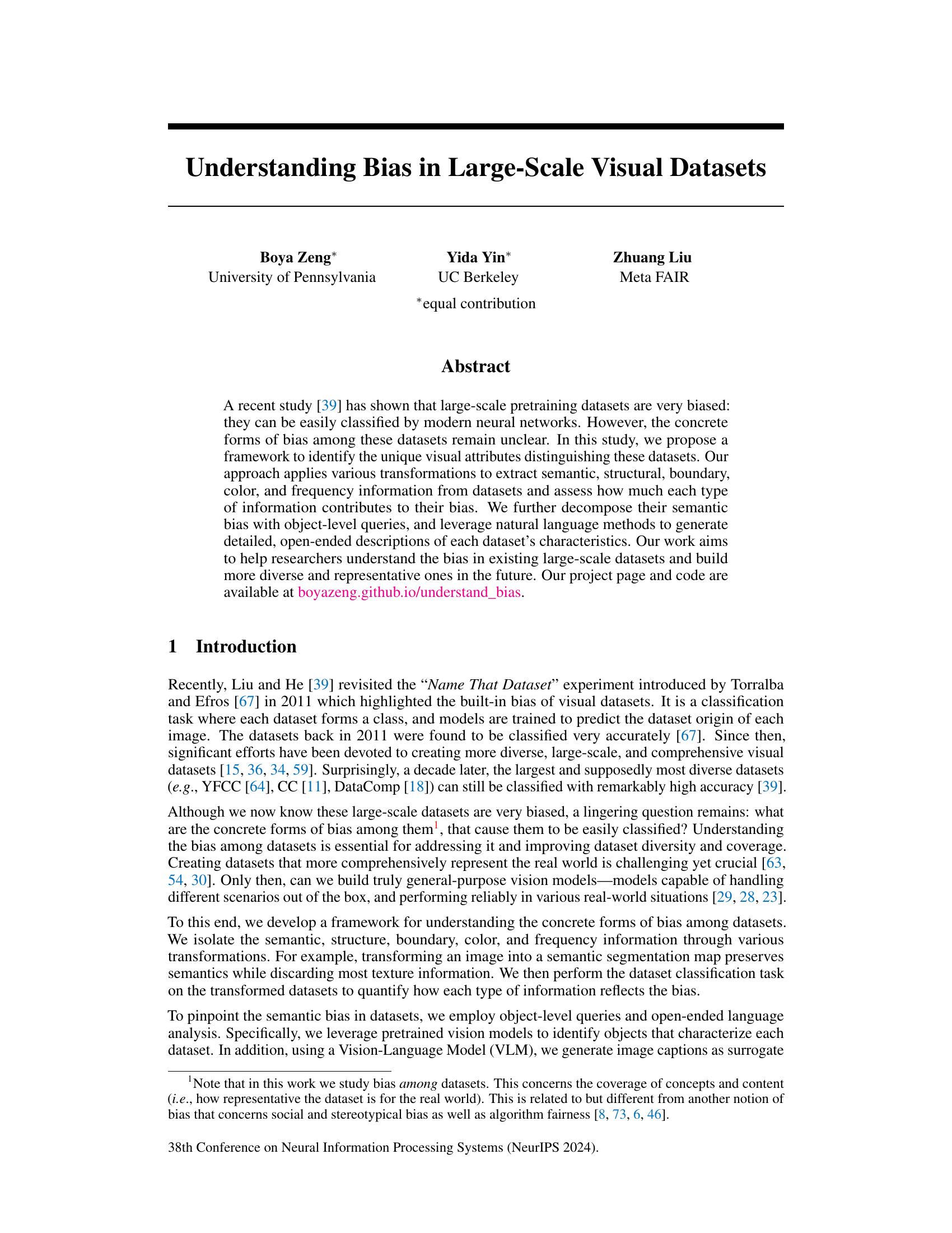
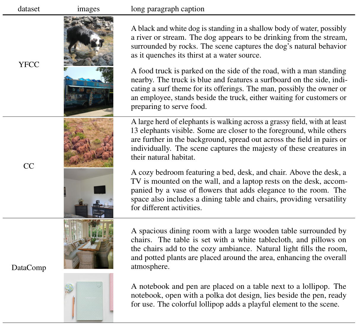
🔼 This figure shows example images from three large-scale visual datasets: YFCC, CC, and DataComp. The purpose is to illustrate the visual differences between these datasets, which are subsequently analyzed in the paper to understand their inherent biases. The caption also notes that a dataset classification model achieves 82% accuracy when classifying images from these datasets based solely on their visual content.
read the caption
Figure 1: Original images. We sample two images from each of YFCC [64], CC [11], and DataComp [18]. Dataset classification on the original images has a reference accuracy of 82.0%.

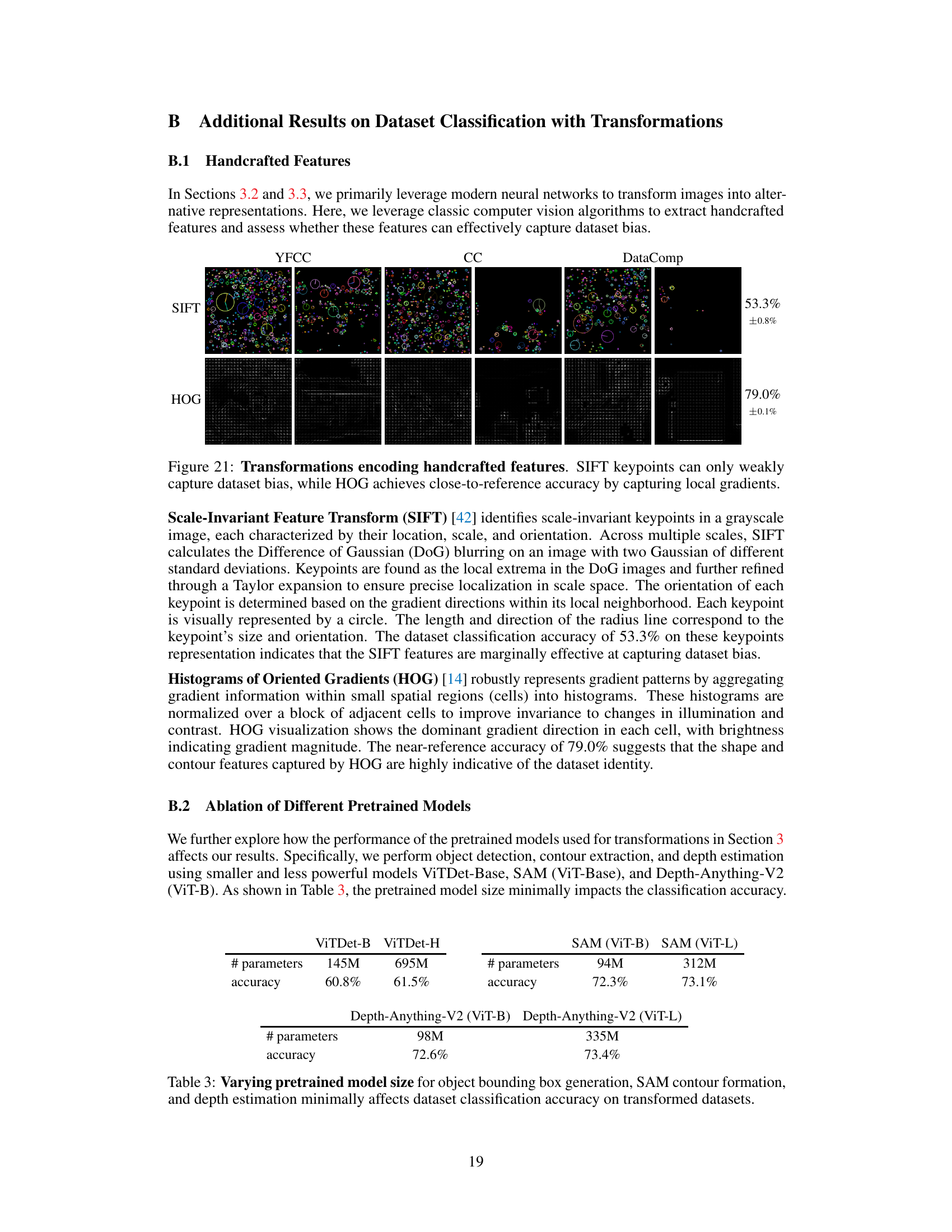
🔼 This table presents the ablation study on the impact of different pretrained model sizes on the performance of object detection, contour extraction, and depth estimation. It shows that using smaller or larger pretrained models (ViTDet-Base vs. ViTDet-Huge, SAM (ViT-Base) vs. SAM (ViT-L), Depth-Anything-V2 (ViT-B) vs. Depth-Anything-V2 (ViT-L)) has minimal impact on the resulting dataset classification accuracy after these transformations, indicating that the choice of pretrained model size does not significantly affect the overall findings of the study.
read the caption
Table 3: Varying pretrained model size for object bounding box generation, SAM contour formation, and depth estimation minimally affects dataset classification accuracy on transformed datasets.
In-depth insights#
Visual Dataset Bias#
Visual dataset bias is a critical issue in computer vision, significantly impacting the fairness, generalizability, and reliability of models trained on these datasets. Bias arises from various sources: including the sampling process, inherent biases in the data collection methods, and skewed representation of certain demographics or visual attributes. This leads to models that perform exceptionally well on specific subsets of the data but poorly generalize to unseen data or real-world scenarios. Understanding the nature of bias is crucial, demanding a multifaceted approach. Research methodologies involve analyzing statistical properties of datasets, examining the impact of specific image features on model performance, and employing advanced techniques like object-level queries and natural language processing to uncover hidden biases. Addressing dataset bias necessitates creating more diverse and representative datasets. This involves thoughtful data collection strategies, careful curation processes that incorporate diverse perspectives and feedback, and developing innovative bias-mitigation algorithms. By creating more inclusive and robust datasets, the field can move towards developing fairer and more reliable computer vision models that benefit a broader range of users.
Bias Quantification#
Bias quantification in large-scale visual datasets is a crucial yet challenging task. A robust methodology needs to move beyond simple classification accuracy and delve into the specific types and degrees of bias present. Identifying the root causes, such as imbalances in object representation, structural biases in image composition, and semantic discrepancies, is vital. This requires a multifaceted approach employing diverse techniques. Data transformations that isolate different visual aspects (e.g., color, texture, shape) are essential for quantifying the contribution of each attribute to overall bias. Statistical analysis should then be applied to the transformed data to generate objective metrics of bias. Natural language processing can analyze image captions and metadata, providing insights into semantic biases and the underlying cultural and social factors that influence dataset composition. Finally, the development of interpretable metrics that communicate bias in an intuitive and readily understandable way to researchers and practitioners is critical for effective bias mitigation.
Transformations#
The core concept of “Transformations” within a visual dataset bias analysis framework involves applying various image manipulations to isolate specific visual attributes and assess their contribution to dataset bias. This systematic approach helps researchers understand the different forms of bias, moving beyond simple dataset classification accuracy. By transforming images into different representations (e.g., semantic segmentation maps, edge detection outlines, color histograms, frequency components), the impact of each visual feature on the model’s ability to distinguish datasets can be isolated and quantified. This controlled experimentation is crucial for a nuanced understanding of bias, as it reveals whether biases are rooted in semantics, structure, color, or texture. The methodology then goes further by leveraging object-level queries and natural language processing techniques to generate detailed descriptions of each dataset’s characteristics, providing an in-depth understanding of how these factors interrelate and contribute to overall dataset bias. The use of transformations is not only insightful, but crucial for building a robust framework, as it provides a comprehensive and methodical way to identify, quantify, and ultimately mitigate biases in large-scale visual datasets, ultimately leading to the development of more representative and inclusive datasets for the future.
Semantic Analysis#
A robust semantic analysis within a research paper would delve into the nuanced meanings conveyed through language. It would move beyond simple keyword identification to explore the relationships between concepts, considering context, synonyms, and potential ambiguities. Effective semantic analysis leverages natural language processing (NLP) techniques such as part-of-speech tagging, named entity recognition, and dependency parsing. These techniques help to identify key entities, their attributes, and relationships, laying the foundation for deeper analysis. Sophisticated methods might incorporate word embeddings and semantic role labeling to better understand the contextual meaning of words and phrases. The ultimate goal is to extract meaningful insights and patterns from the text, going beyond the surface level to uncover the underlying meaning. A successful approach will consider various aspects like sentiment analysis, topic modeling, and the identification of key themes or arguments. The insights gleaned from such an analysis can significantly contribute to the overall interpretation and understanding of the research paper, providing a deeper understanding of the author’s arguments and their implications.
Future Datasets#
A thoughtful consideration of “Future Datasets” in research necessitates a multi-faceted approach. Firstly, future datasets should prioritize diversity and inclusivity, actively addressing historical biases in representation. This involves careful consideration of demographic factors, geographical locations, and cultural contexts to ensure a more representative sample of the real world. Secondly, the development of robust and reliable methods for evaluating dataset quality is crucial. This requires the creation of standardized metrics and procedures that go beyond simple quantitative measures to incorporate qualitative assessments of fairness, representativeness, and utility. Thirdly, the sustainability of future datasets should be a paramount concern. This includes adopting data management practices that ensure long-term accessibility, usability, and preservation of data, even with changing technological landscapes. Finally, the ethical implications of data collection and utilization must be carefully considered. This means developing transparent and accountable frameworks for data governance and ensuring compliance with relevant regulations and ethical guidelines.
More visual insights#
More on figures
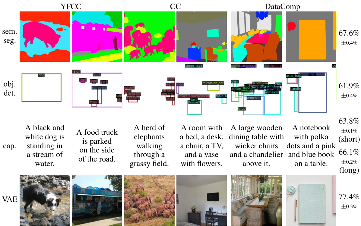
🔼 This figure shows the results of applying different image transformations to three large-scale visual datasets (YFCC, CC, and DataComp) before performing dataset classification. The transformations include semantic segmentation, object detection, image captioning, and Variational Autoencoder (VAE). The results show that even after these transformations, which either preserve or reduce specific aspects of visual information, the dataset classification accuracy remains high. This indicates that semantic differences (the meaning of the images) are a key driver of the bias in these datasets, rather than just low-level visual features (e.g. color, texture).
read the caption
Figure 2: Transformations preserving semantic information (semantic segmentation, object detection, and caption) and potentially reducing low-level signatures (VAE) result in high dataset classification accuracy. This suggests that semantic discrepancy is an important form of dataset bias.
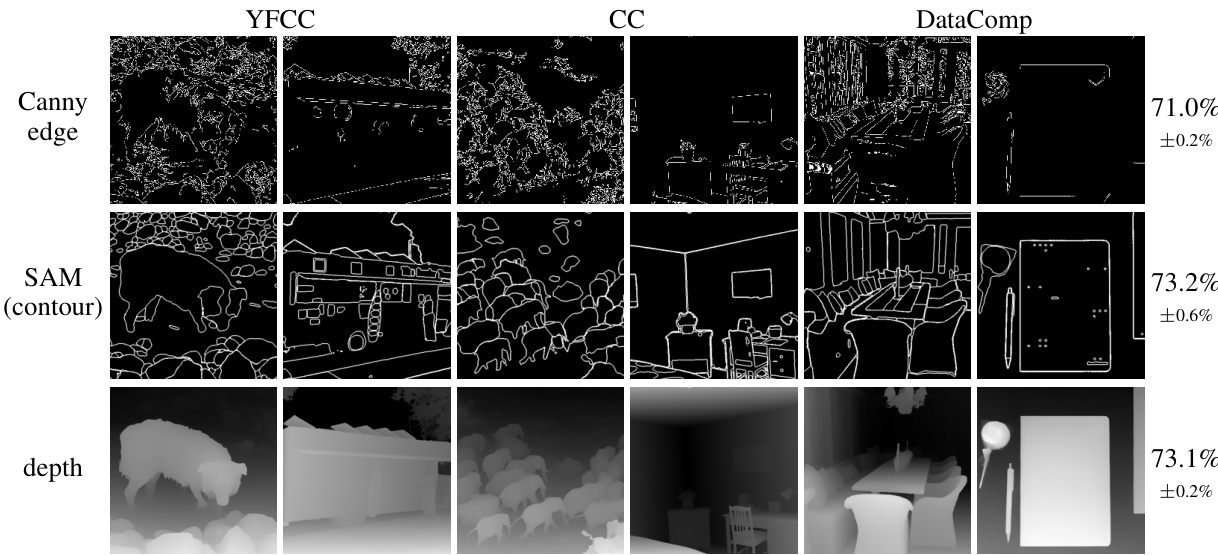
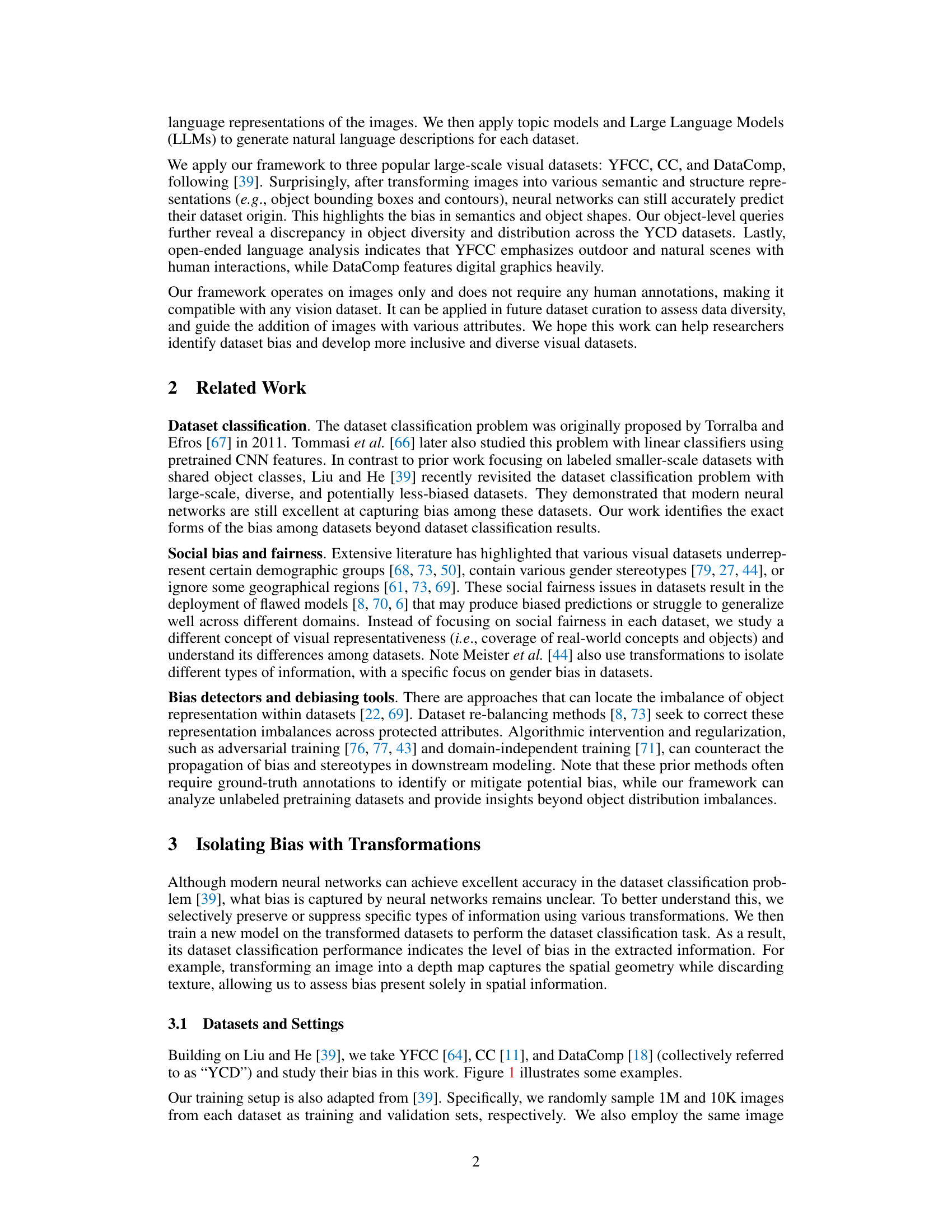
🔼 This figure shows the results of applying different image transformations to isolate structural information (object shapes and spatial geometry) and then performing dataset classification. The transformations used include Canny edge detection, Segment Anything Model (SAM) for contour extraction, and depth estimation. The results indicate that even after removing semantic information, the models can still accurately classify the datasets, suggesting significant differences in object shapes and spatial structures across datasets.
read the caption
Figure 3: Transformations outlining object shapes and estimating pixel depth. Dataset classification achieves even higher accuracies on object contours and depth images than on semantic information, indicating that object shapes and spatial geometry vary significantly across YCD.
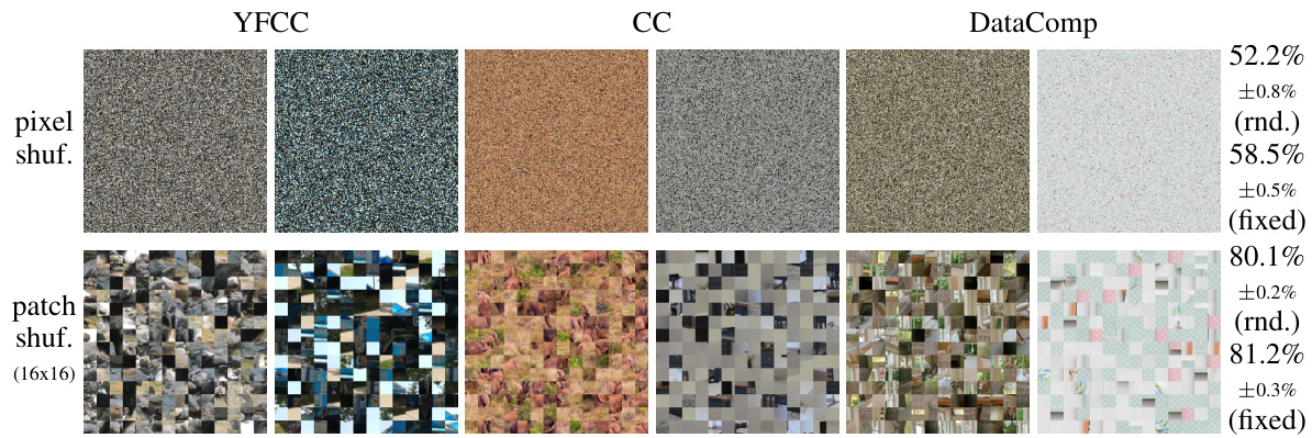
🔼 This figure shows the results of applying pixel and patch shuffling transformations to the images of three datasets (YFCC, CC, and DataComp). Pixel shuffling randomly shuffles the pixels within each image, destroying the spatial structure. Patch shuffling divides the image into patches and shuffles their order, preserving some local spatial structure. The classification accuracy is significantly lower after pixel shuffling, but relatively high after patch shuffling. This demonstrates that models learn dataset-specific patterns from the local spatial structure within the images, rather than global patterns.
read the caption
Figure 4: Transformations breaking spatial structure. Pixel shuffling drastically decreases dataset classification accuracy, but patch shuffling has minimal impact. This demonstrates that local structure is important and sufficient for models to learn the patterns of each dataset.

🔼 This figure shows the impact of varying patch sizes on the accuracy of dataset classification after patch shuffling. The x-axis represents different patch sizes (1, 2, 4, 8, 16), and the y-axis shows the classification accuracy. Two lines are plotted: one for randomly shuffled patches and one for patches shuffled in a fixed order. A horizontal dashed line indicates the reference accuracy on the original images. As patch size increases, the accuracy of both random and fixed order shuffling approaches the reference accuracy, suggesting that larger patches preserve more spatial information crucial for dataset classification.
read the caption
Figure 5: Effect of patch sizes. Accuracy approaches the reference one with larger patch sizes.

🔼 This figure shows the average RGB values for each dataset (YFCC, CC, and DataComp). Even though all color information is reduced to a single average color value per image, the model can still classify the images into their respective datasets with a non-trivial accuracy of 48.5%. This indicates that there are color distribution differences between the datasets, and these differences contribute to the model’s ability to distinguish between the datasets.
read the caption
Figure 6: Averaging each color channel. Even when the values of each channel in images are averaged, the model can still achieve non-trivial dataset classification performance.

🔼 This figure displays the distribution of mean RGB values for the three datasets (YFCC, CC, DataComp) and their confusion matrix after dataset classification using only mean RGB values. The distributions show that YFCC images have lower RGB values overall than CC and DataComp, which have similar distributions. The confusion matrix shows that YFCC images are easily classified correctly, but CC and DataComp images are often confused with each other.
read the caption
Figure 7: Distribution of mean RGB values and confusion matrix. YFCC's RGB values are overall smaller, while CC's and DataComp's are very similar. This is also reflected in the confusion matrix of dataset classification on mean RGB images, where YFCC can be classified very easily (indicated by the dark blue box on the top left), while there is high confusion between CC and DataComp.

🔼 This figure displays the results of applying high-pass and low-pass filters to images from the YFCC, CC, and DataComp datasets. The top row shows the low-pass filtered images, and the bottom row shows the high-pass filtered images. Each column represents one dataset. The high-pass filtered images are equalized for better visualization. The caption indicates that the accuracy of dataset classification remains close to the reference accuracy, even after applying these filters. This suggests that the dataset bias is present across different frequencies (high and low).
read the caption
Figure 8: Transformations filtering high-frequency and low-frequency components retain close-to-reference accuracy. This indicates that dataset bias exists in different frequencies. The high-pass filtered images are equalized for better visualization.

🔼 This figure shows example images generated by unconditional and text-to-image diffusion models, trained on the three datasets YFCC, CC, and DataComp. The top row displays images generated using an unconditional model (meaning the model generated images without any text prompt), and it shows that the resulting images still retain enough characteristics of their original dataset to be easily classified. The bottom row shows images generated using a text-to-image model (meaning the model used a text description as a prompt to generate the image), and these images, while still showing some bias towards their original dataset, are harder to classify than the unconditionally generated images. This suggests that semantic information (carried by the text description in the text-to-image model) plays a significant role in the bias observed in large-scale visual datasets.
read the caption
Figure 9: Synthetic images from unconditional and text-to-image generation models. Unconditionally generated images can be classified with near-reference accuracy. Images from text-to-image diffusion models using short captions have reasonable dataset classification accuracy.

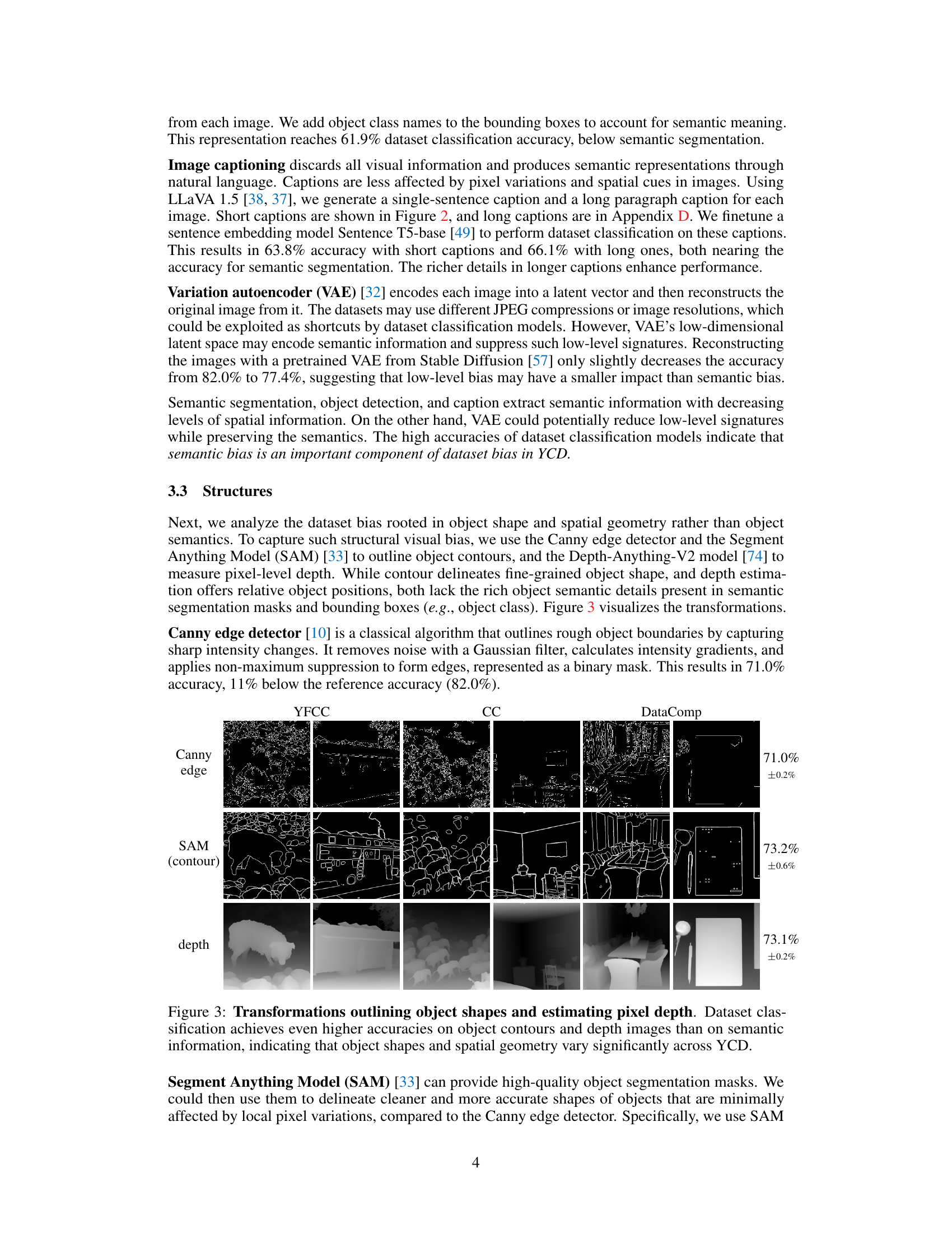
🔼 Grad-CAM highlights image regions influencing the model’s dataset classification predictions. The figure shows Grad-CAM heatmaps for the dataset classification model applied to images from YFCC, CC, and DataComp. The heatmaps reveal that the model attends to semantically meaningful objects (e.g., an elephant herd, table and chairs, pen) to predict the dataset origin. This illustrates that the model leverages object-level information for accurate dataset classification, suggesting a strong dependence on semantic bias.
read the caption
Figure 10: Grad-CAM heatmap [80, 60] on the dataset classification model trained on original datasets. It focuses on specific objects to determine the dataset origin of each image.

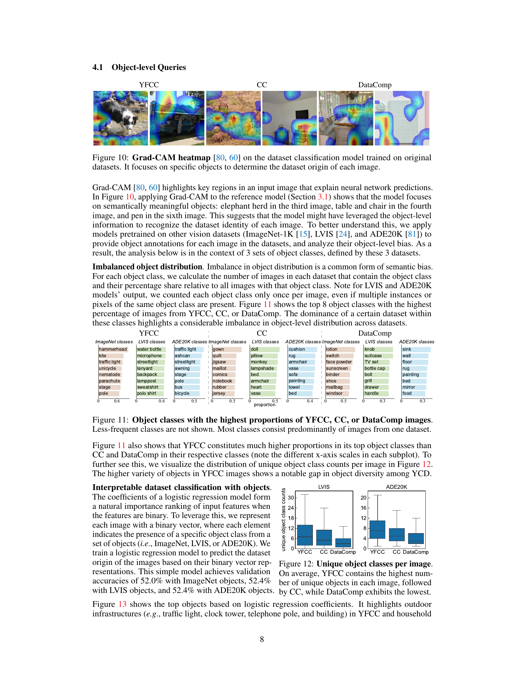
🔼 This figure visualizes the imbalance in object-level distribution across three large-scale visual datasets: YFCC, CC, and DataComp. For each dataset, it shows the top eight object classes that have the highest percentage of images from that dataset. The significant dominance of a single dataset within many of these classes highlights a substantial imbalance in object distribution, indicating a key aspect of semantic bias among the datasets. The x-axis scales differ across subplots to better represent the varied distributions.
read the caption
Figure 11: Object classes with the highest proportions of YFCC, CC, or DataComp images. Less-frequent classes are not shown. Most classes consist predominantly of images from one dataset.

🔼 This figure uses boxplots to show the distribution of the number of unique object classes per image for three large-scale visual datasets: YFCC, CC, and DataComp. The Y-axis represents the number of unique object classes, and the X-axis represents the datasets. Each boxplot shows the median, quartiles, and outliers of the distribution. The figure illustrates that YFCC images tend to contain a higher number of unique object classes compared to CC and DataComp images, which have relatively fewer unique object classes per image. This indicates a difference in the diversity of objects present across these three datasets, suggesting a potential bias towards a narrower range of visual concepts in CC and DataComp.
read the caption
Figure 12: Unique object classes per image. On average, YFCC contains the highest number of unique objects in each image, followed by CC, while DataComp exhibits the lowest.
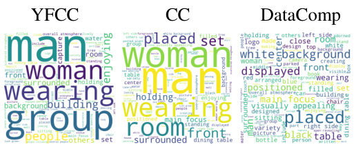
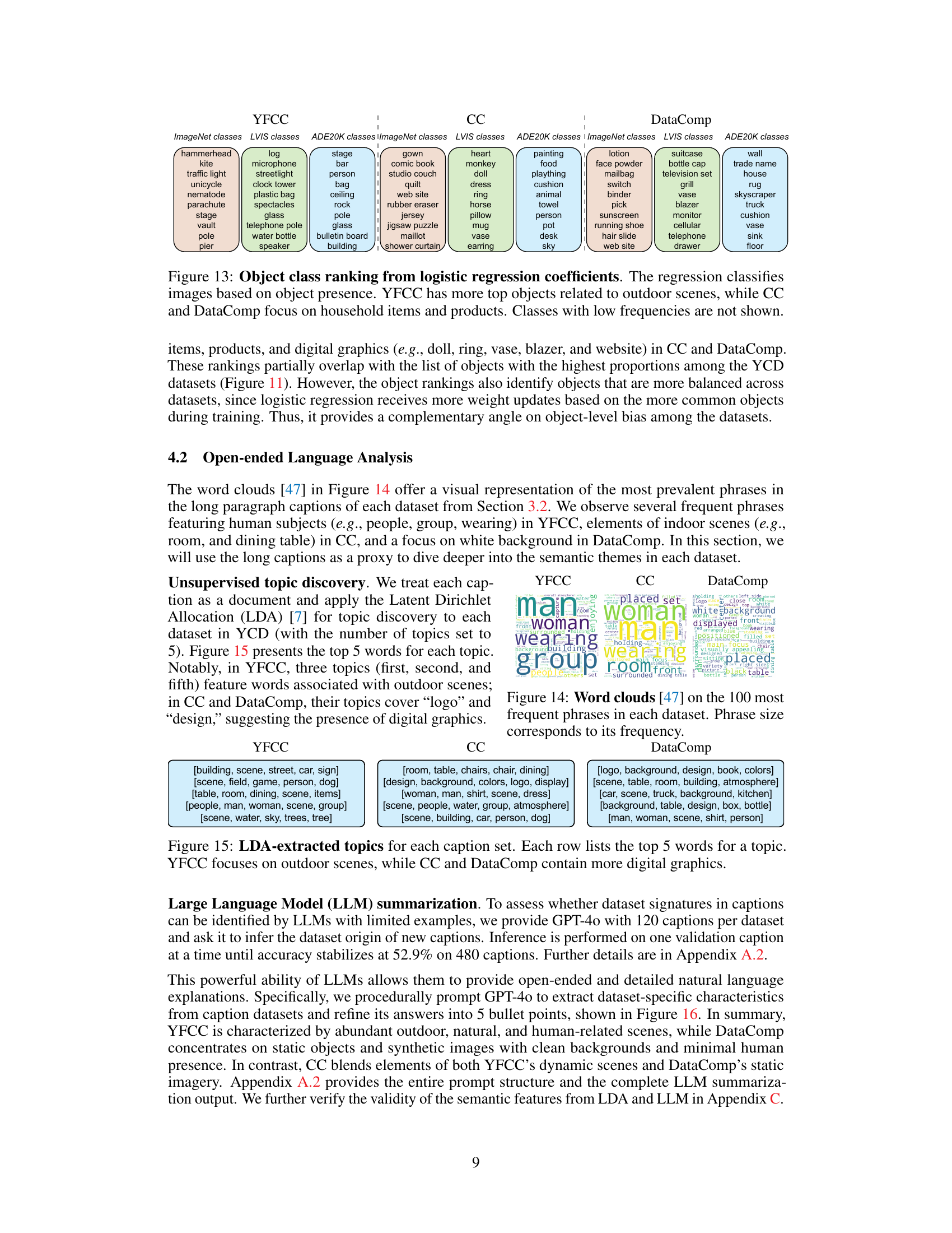
🔼 This figure shows word clouds generated from the captions of each dataset. The size of each word corresponds to its frequency of appearance in the captions. It visually summarizes the main themes or topics present in the captions of each dataset, providing a quick overview of their semantic characteristics. YFCC focuses on outdoor scenes and human activities, CC shows words related to indoor scenes and human interactions, and DataComp emphasizes product descriptions and digital graphics.
read the caption
Figure 14: Word clouds [47] on the 100 most frequent phrases in each dataset. Phrase size corresponds to its frequency.

🔼 This figure displays two sample images from each of the three large-scale visual datasets: YFCC, CC, and DataComp. These images are representative of the types of images found in each dataset. The caption notes that a dataset classification model achieves 82% accuracy when classifying images from these three datasets, indicating significant bias within the datasets, making them easily distinguishable from one another.
read the caption
Figure 1: Original images. We sample two images from each of YFCC [64], CC [11], and DataComp [18]. Dataset classification on the original images has a reference accuracy of 82.0%.

🔼 This figure displays two sample images from each of the three large-scale visual datasets used in the study: YFCC, CC, and DataComp. The purpose is to visually illustrate the diversity (or lack thereof) in these datasets before applying various transformations and analyses. The caption also notes that a dataset classification model achieves 82% accuracy when classifying images from these datasets based on their source dataset alone, highlighting the significant bias embedded in these large-scale datasets.
read the caption
Figure 1: Original images. We sample two images from each of YFCC [64], CC [11], and DataComp [18]. Dataset classification on the original images has a reference accuracy of 82.0%.

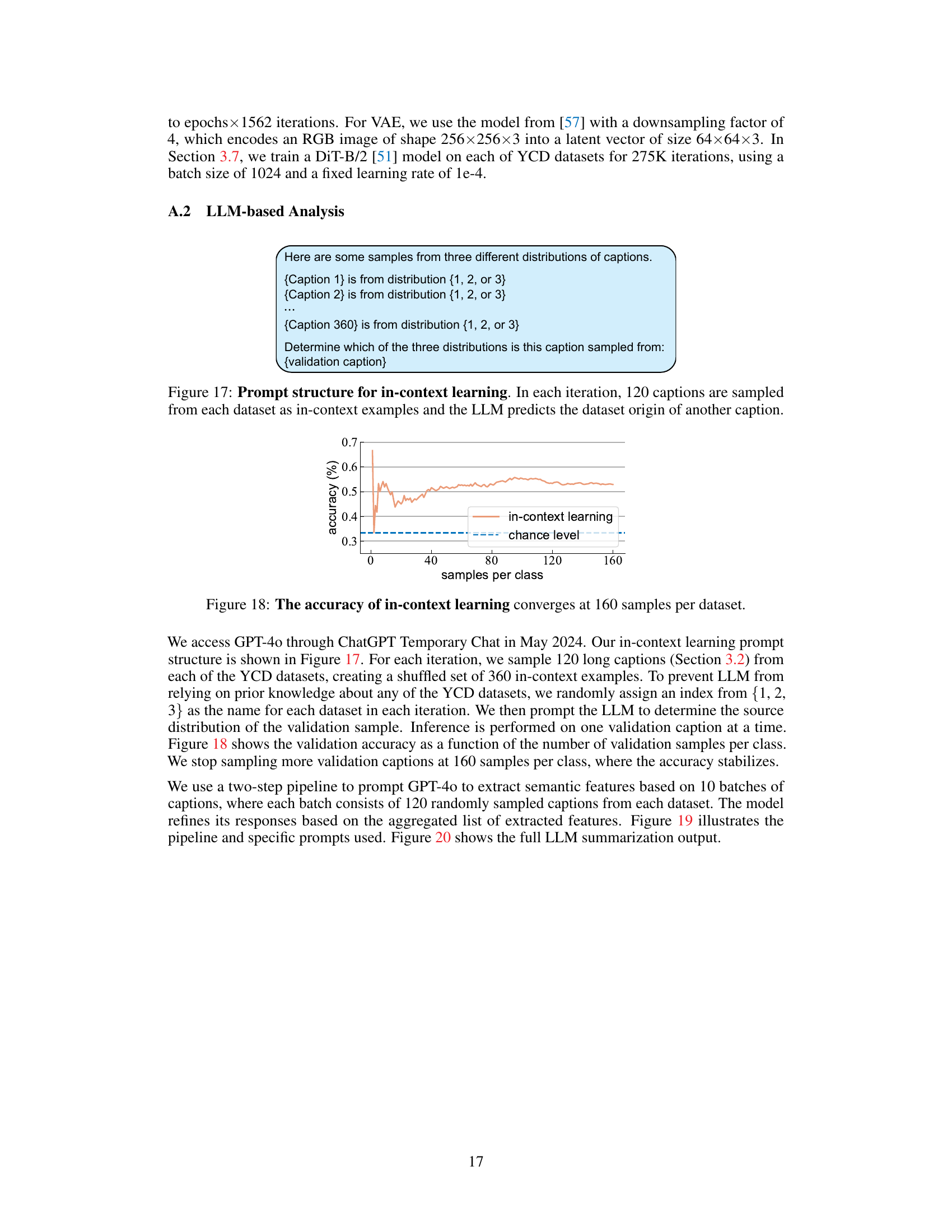
🔼 The figure shows the accuracy of in-context learning using GPT-40, as the number of samples per class increases. The accuracy gradually increases and stabilizes around 0.55 after about 160 samples per class, exceeding the chance level of 0.33. This indicates that with sufficient in-context examples, the LLM can effectively learn to classify the dataset origin of captions.
read the caption
Figure 18: The accuracy of in-context learning converges at 160 samples per dataset.

🔼 This figure shows two sample images from each of the three large-scale visual datasets used in the study: YFCC, CC, and DataComp. The purpose is to visually demonstrate the diversity (or lack thereof) in image content across the different datasets. The caption also notes that a baseline model achieves 82% accuracy in classifying images to their source dataset, highlighting the existence of significant bias.
read the caption
Figure 1: Original images. We sample two images from each of YFCC [64], CC [11], and DataComp [18]. Dataset classification on the original images has a reference accuracy of 82.0%.
🔼 This figure displays two sample images from each of the three large-scale visual datasets: YFCC, CC, and DataComp. The purpose is to visually illustrate the types of images contained within each dataset. The caption also notes that a dataset classification model achieved 82% accuracy when trained on these images, establishing a baseline for later comparisons using transformed images.
read the caption
Figure 1: Original images. We sample two images from each of YFCC [64], CC [11], and DataComp [18]. Dataset classification on the original images has a reference accuracy of 82.0%.

🔼 This figure shows the results of using handcrafted features, Scale-Invariant Feature Transform (SIFT) and Histograms of Oriented Gradients (HOG), for dataset classification. SIFT keypoints, visualized as circles with orientations, show weak ability to distinguish between datasets, achieving only 53.3% accuracy. HOG features, visualizing gradient orientations and magnitudes, perform significantly better, achieving 79.0% accuracy, demonstrating that local gradient information is strongly indicative of dataset bias.
read the caption
Figure 21: Transformations encoding handcrafted features. SIFT keypoints can only weakly capture dataset bias, while HOG achieves close-to-reference accuracy by capturing local gradients.

🔼 This figure displays two example images from each of the three large-scale visual datasets used in the study: YFCC, CC, and DataComp. These datasets are the focus of the bias analysis. The caption notes that a dataset classification model achieves 82% accuracy when trained on these original images, serving as a baseline for comparison with results from transformed images in later experiments. This baseline indicates the strong inherent bias within the datasets, as the model can easily distinguish between their image styles.
read the caption
Figure 1: Original images. We sample two images from each of YFCC [64], CC [11], and DataComp [18]. Dataset classification on the original images has a reference accuracy of 82.0%.
🔼 This figure shows two example images from each of the three large-scale visual datasets used in the paper: YFCC, CC, and DataComp. The purpose is to illustrate the visual diversity (or lack thereof) in the datasets. The caption also notes that a baseline dataset classification model achieves 82% accuracy on these images, highlighting the bias present in the datasets that allows for such high accuracy.
read the caption
Figure 1: Original images. We sample two images from each of YFCC [64], CC [11], and DataComp [18]. Dataset classification on the original images has a reference accuracy of 82.0%.
🔼 This figure shows two example images from each of the three large-scale visual datasets used in the study: YFCC, CC, and DataComp. The purpose is to visually illustrate the diversity (or lack thereof) within and between the datasets, which is a central theme of the paper. The caption also notes that a baseline dataset classification model achieves 82% accuracy when trained on these original images, providing a benchmark for comparison with the results obtained using various image transformations.
read the caption
Figure 1: Original images. We sample two images from each of YFCC [64], CC [11], and DataComp [18]. Dataset classification on the original images has a reference accuracy of 82.0%.

🔼 This figure shows the results of applying ideal high-pass and low-pass filters to images with different threshold values. The thresholds used are 5, 35, 65, 95, 125, and 155. The top row displays the low-pass filtered images, which are progressively more blurred as the threshold increases. The bottom row contains the high-pass filtered images, showcasing increasingly prominent edge details as the threshold value increases. This visualization helps to demonstrate how different frequency components of images contribute to the overall visual information. The high-pass images are equalized to enhance visibility.
read the caption
Figure 24: Ideal filter [21] with different thresholds. We select filtering thresholds {5, 35, 65, 95, 125, 155}. The high-pass filtered images are equalized for better visualization.

🔼 This figure shows the results of applying Butterworth filters with different thresholds (5, 35, 65, 95, 125, 155) to images. The top row displays low-pass filtered images, showing a gradual increase in detail as the threshold increases. The bottom row displays high-pass filtered images, highlighting edges and textures. The equalization of the high-pass filtered images helps to improve visibility.
read the caption
Figure 25: Butterworth filter [9] with different thresholds. We select filtering thresholds {5, 35, 65, 95, 125, 155}. The high-pass filtered images are equalized for better visualization.

🔼 This figure shows the accuracy of dataset classification on images filtered using ideal and Butterworth filters, with different thresholds applied. The x-axis represents the filter threshold, while the y-axis shows the accuracy. Two lines are plotted for each filter type (low-pass and high-pass), and a horizontal line shows the reference accuracy without filtering. The results indicate that using both filter types across a range of thresholds yields high accuracies close to the reference, suggesting the dataset bias is present in both low and high frequency information.
read the caption
Figure 26: Accuracy on filtered images at different thresholds. For most thresholds, both ideal and Butterworth filters achieve high accuracies for both high-pass and low-pass filters.

🔼 The figure shows the results of using LLaVA, a vision-language model, to identify high-level semantic features in the YFCC, CC, and DataComp datasets. Five features were tested: whether the image is a product showcase, has an entirely white background, depicts a person, shows an outdoor scene, or a domestic scene. For each feature and dataset, the percentage of images where the feature is present is shown. The results confirm the semantic biases identified in Section 4.2 of the paper, demonstrating differences in the types of images each dataset contains.
read the caption
Figure 27: High-level semantic features' distributions annotated by LLaVA. The imbalanced distributions across YCD confirm the dataset characteristics in Section 4.2.

🔼 This figure shows two example images from each of the three datasets: YFCC, CC, and DataComp. The purpose is to visually illustrate the differences in image content and style across the datasets. The caption notes that a dataset classification model achieves 82% accuracy when classifying these images based solely on their source dataset.
read the caption
Figure 1: Original images. We sample two images from each of YFCC [64], CC [11], and DataComp [18]. Dataset classification on the original images has a reference accuracy of 82.0%.

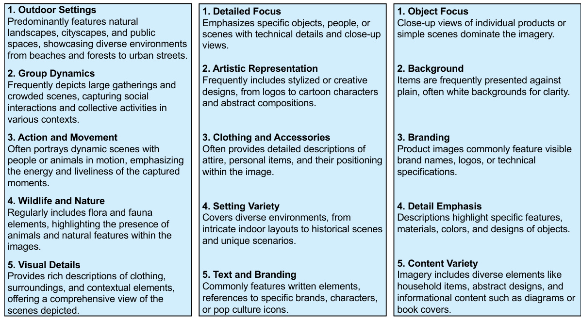
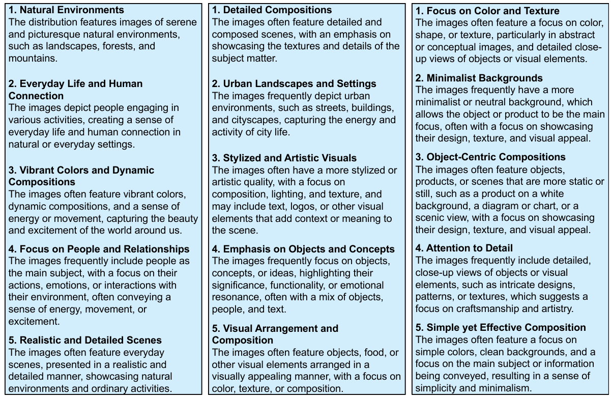
🔼 This figure displays a table summarizing the key features that distinguish the three datasets (YFCC, CC, and DataComp) from each other, as determined by the VisDiff method. The analysis focuses on identifying high-level concepts that differentiate the datasets’ visual content. Each cell in the table shows the top 3 concepts that distinguish one dataset from another. The concepts identified by VisDiff align well with the semantic characteristics found through the language analysis performed earlier in Section 4.2 of the paper, indicating consistency in the methods of determining semantic differences.
read the caption
Figure 28: Dataset features generated by VisDiff [17]. Each cell lists the top 3 concepts distinguishing the dataset in each column from the one in each row. Note the VisDiff concepts highly overlap with the dataset characteristics from our language analysis in Section 4.2.
🔼 This figure shows two sample images from each of the three large-scale visual datasets used in the study: YFCC, CC, and DataComp. The purpose is to visually illustrate the diversity (or lack thereof) present in these datasets. The caption also notes that a baseline dataset classification model achieves 82% accuracy when trained on these original images, serving as a benchmark for comparison against the accuracy achieved using transformed images in later experiments.
read the caption
Figure 1: Original images. We sample two images from each of YFCC [64], CC [11], and DataComp [18]. Dataset classification on the original images has a reference accuracy of 82.0%.
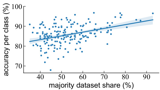
🔼 This figure shows a positive correlation between the majority dataset share of an ImageNet object class and the accuracy of the reference dataset classification model for that class. In other words, object classes predominantly found in a single dataset tend to have higher classification accuracy in predicting the dataset origin of images where they appear. This suggests that dataset bias heavily influences the model’s ability to accurately predict dataset sources based on individual object classes.
read the caption
Figure 29: Majority dataset share for each ImageNet object class positively correlates with the reference dataset classification accuracy on that object class.
More on tables

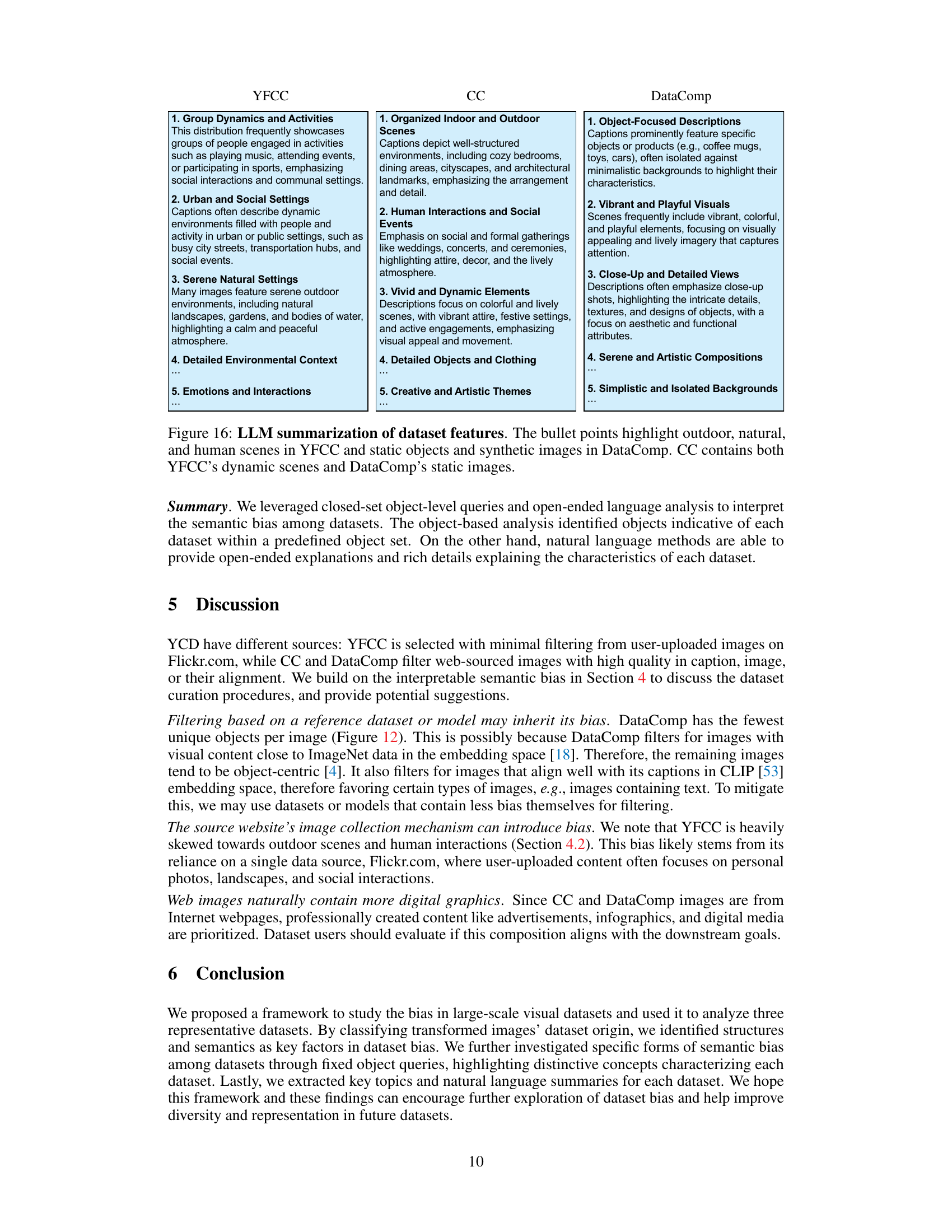
🔼 This table presents the top 5 words for each topic extracted by Latent Dirichlet Allocation (LDA) from captions of three datasets: YFCC, CC, and DataComp. The topics reveal the predominant themes in each dataset’s captions. YFCC’s topics strongly emphasize outdoor settings and activities, while CC’s show a mix of indoor and outdoor settings. DataComp’s topics highlight digital graphics, design elements, and product descriptions.
read the caption
Table 15: LDA-extracted topics for each caption set. Each row lists the top 5 words for a topic. YFCC focuses on outdoor scenes, while CC and DataComp contain more digital graphics.

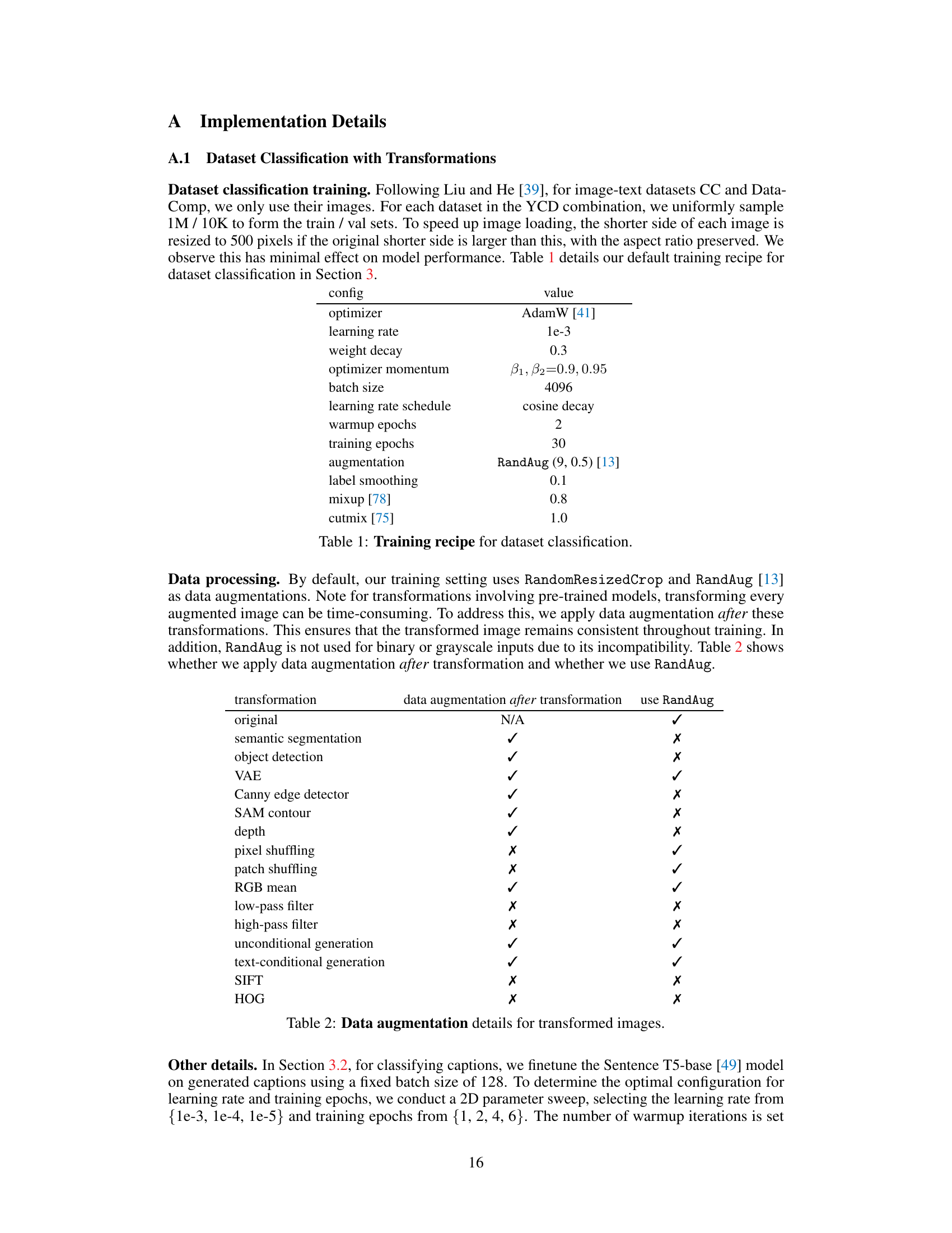
🔼 This table details the training settings used for the dataset classification task in Section 3 of the paper. It specifies the optimizer (AdamW), learning rate (1e-3), weight decay (0.3), optimizer momentum (β1, β2=0.9, 0.95), batch size (4096), learning rate schedule (cosine decay), warmup epochs (2), training epochs (30), augmentations (RandAug (9, 0.5)), label smoothing (0.1), mixup (0.8), and cutmix (1.0).
read the caption
Table 1: Training recipe for dataset classification.

🔼 This table indicates whether data augmentation was applied after image transformations and whether RandAug was used for each type of transformation. Data augmentation was not applied for binary or grayscale images due to incompatibility with RandAug. RandAug was used for most transformations except for those producing binary, grayscale, or other forms of non-standard images.
read the caption
Table 2: Data augmentation details for transformed images.
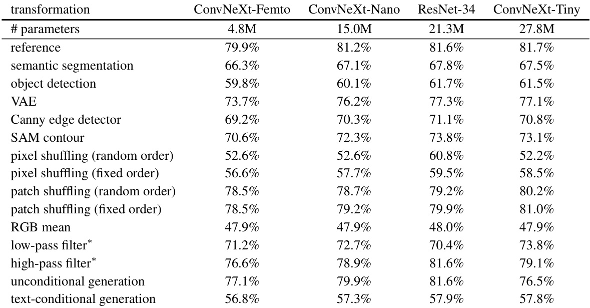
🔼 This table presents the results of dataset classification accuracy using four different vision backbones (ConvNeXt-Femto, ConvNeXt-Nano, ResNet-34, and ConvNeXt-Tiny) on various image transformations. The purpose is to demonstrate the robustness of the findings in the paper by showing consistent accuracy across various models. The results show that even with different model architectures and sizes, the classification accuracy on the transformed images remains relatively consistent, indicating that the observed bias is not an artifact of the specific model used.
read the caption
Table 4: Different image classification models' validation accuracy on transformed datasets. The accuracy remains consistent across models and transformations. * Note the frequency filters here are Butterworth filters [9] with a threshold of 30.

🔼 This table presents the results of an ablation study investigating the impact of different pretrained model sizes on the accuracy of dataset classification using various image transformations. The transformations considered include object bounding box generation, SAM contour formation, and depth estimation. The results show that varying the size of the pretrained models used for these transformations has minimal impact on the classification accuracy, suggesting that the overall effectiveness of the transformations is not strongly dependent on model size.
read the caption
Table 3: Varying pretrained model size for object bounding box generation, SAM contour formation, and depth estimation minimally affects dataset classification accuracy on transformed datasets.

🔼 This table presents the results of dataset classification experiments where multiple image transformations were combined. Specifically, it shows the accuracy achieved when using two transformations together (e.g., pixel shuffling and object detection) compared to using each transformation individually. The results demonstrate that combining certain types of transformations can lead to significantly higher accuracy in predicting the dataset of origin, indicating that these combined visual attributes contribute to a larger dataset bias.
read the caption
Table 6: Combination of different transformations can lead to larger bias.

🔼 This table presents the training accuracy for pseudo-dataset classification on YFCC bounding boxes, with and without augmentations. The results show that the model fails to generalize beyond the training data when more images or strong augmentations are used, indicating that the model is memorizing the training data rather than learning generalizable patterns.
read the caption
Table 7: Training accuracy for YFCC bounding box pseudo dataset classification.
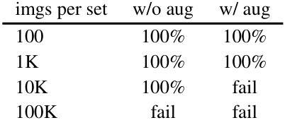
🔼 This table presents the results of training a model to classify pseudo-datasets created from the YFCC dataset’s bounding boxes. The pseudo-datasets were created by sampling from the transformed YFCC bounding boxes without replacement. The table shows the training accuracy with and without augmentations for different sizes of pseudo-datasets. The purpose is to evaluate if the model generalizes or simply memorizes.
read the caption
Table 7: Training accuracy for YFCC bounding box pseudo dataset classification.
Full paper#
