TL;DR#
Deep learning models often prioritize simpler features, potentially leading to shortcut learning and poor generalization. This hinders the development of robust and interpretable AI systems. Existing methods for assessing feature complexity are limited and lack a computational perspective.
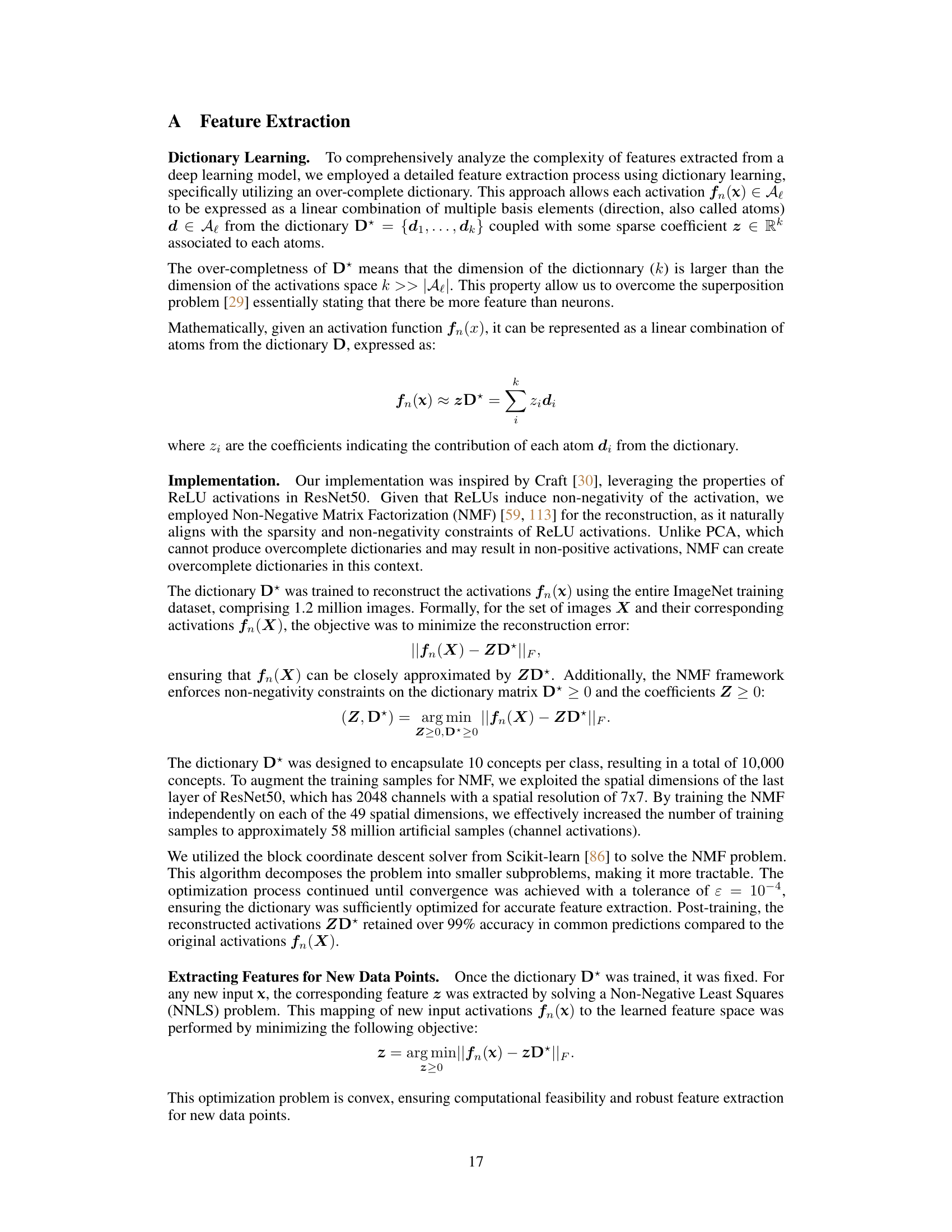
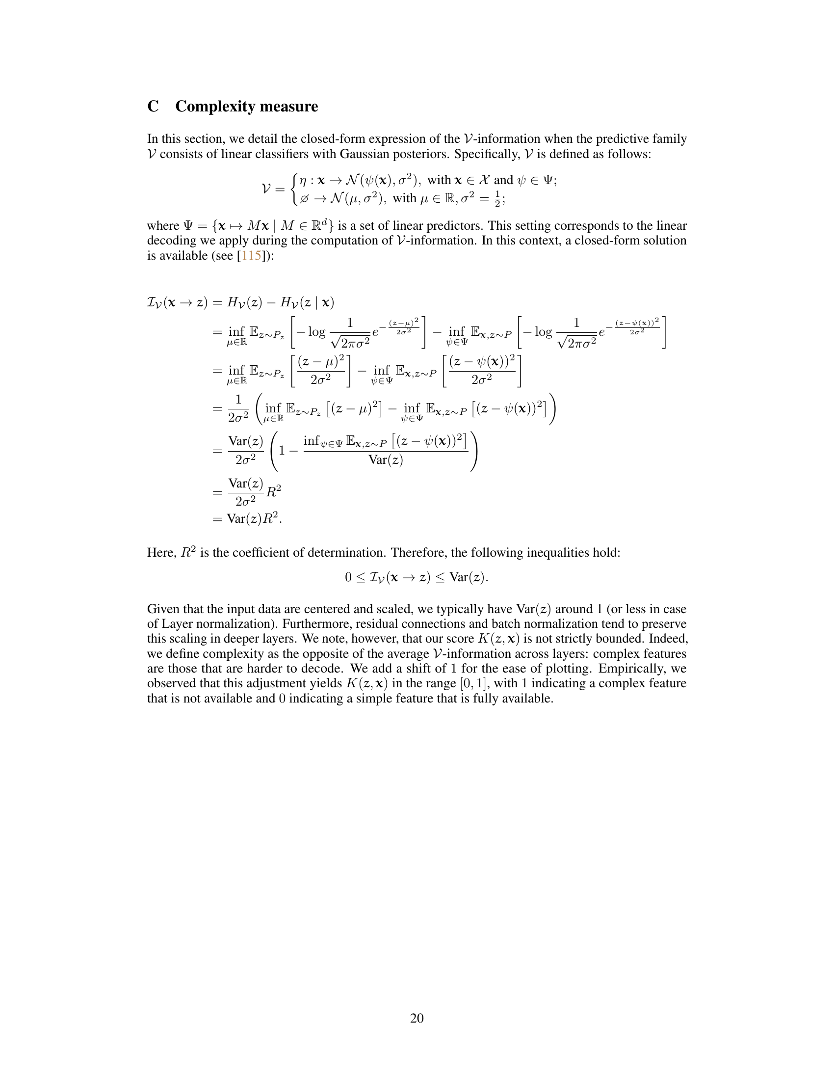
This work presents a novel V-information-based metric to quantify feature complexity, analyzing features extracted from a ResNet50 model trained on ImageNet. The study investigates the relationship between feature complexity, their learning timing, location within the network, and their importance in driving model predictions. It finds that simpler features are learned early and tend to use residual connections, while more complex features emerge later but are less influential in decision-making. Importantly, the model simplifies its most important features over time. This research provides crucial insights into feature learning dynamics and challenges assumptions about the role of complex features in model performance.
Key Takeaways#
Why does it matter?#
This paper is crucial for researchers working on explainable AI, deep learning model interpretability, and shortcut learning. It introduces a novel complexity metric and provides valuable insights into feature learning dynamics, paving the way for more robust and interpretable models. The findings challenge existing assumptions about feature importance and suggest new avenues for research, particularly concerning the balance between simplicity and complexity in model development.
Visual Insights#

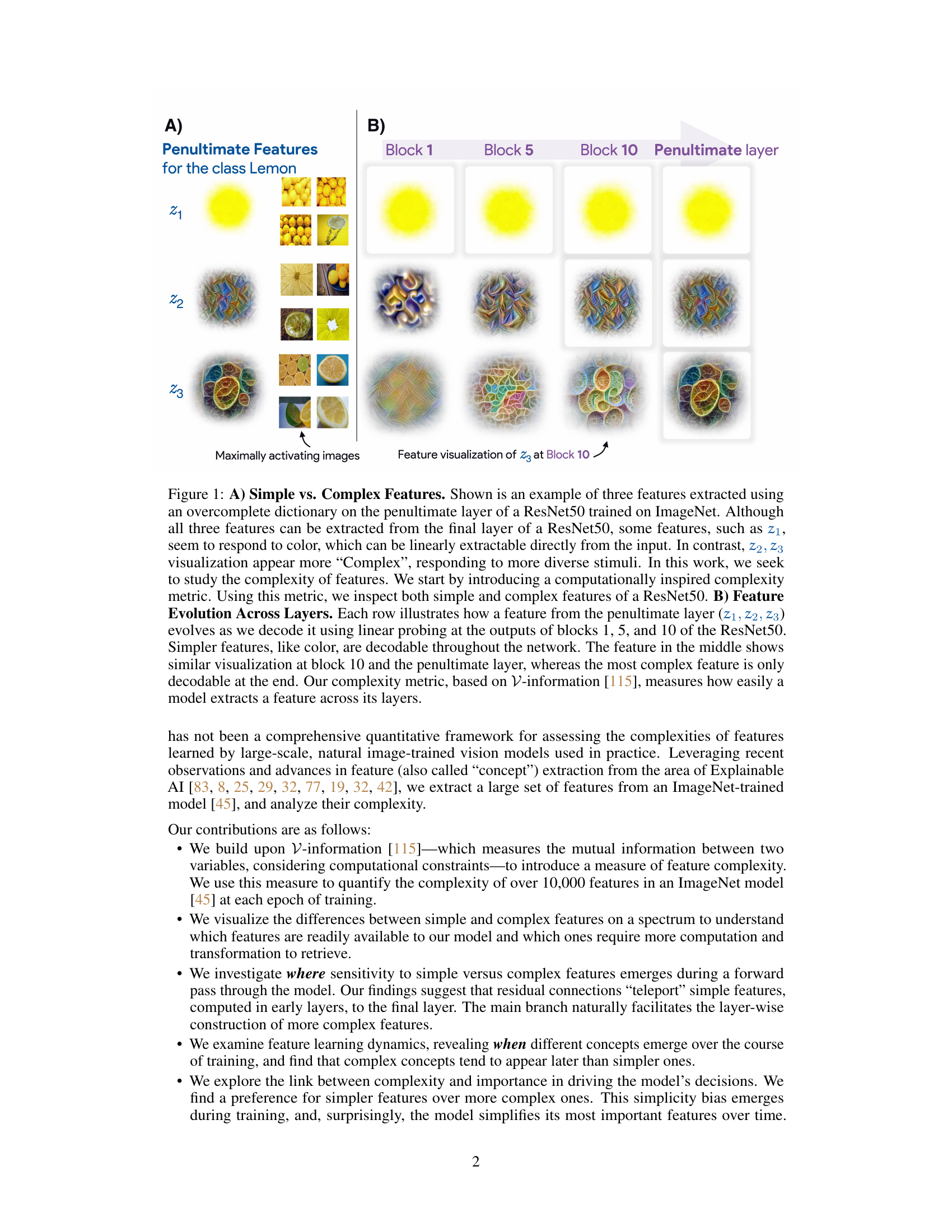
🔼 This figure shows examples of simple and complex features extracted from a ResNet50 model trained on ImageNet. Panel A illustrates that simpler features (e.g., color) can be easily extracted from early layers, while complex features require deeper processing. Panel B demonstrates how features evolve across different layers of the network, with simple features remaining consistent and complex features emerging gradually.
read the caption
Figure 1: A) Simple vs. Complex Features. Shown is an example of three features extracted using an overcomplete dictionary on the penultimate layer of a ResNet50 trained on ImageNet. Although all three features can be extracted from the final layer of a ResNet50, some features, such as z1, seem to respond to color, which can be linearly extractable directly from the input. In contrast, z2, z3 visualization appear more 'Complex', responding to more diverse stimuli. In this work, we seek to study the complexity of features. We start by introducing a computationally inspired complexity metric. Using this metric, we inspect both simple and complex features of a ResNet50. B) Feature Evolution Across Layers. Each row illustrates how a feature from the penultimate layer (z1, z2, z3) evolves as we decode it using linear probing at the outputs of blocks 1, 5, and 10 of the ResNet50. Simpler features, like color, are decodable throughout the network. The feature in the middle shows similar visualization at block 10 and the penultimate layer, whereas the most complex feature is only decodable at the end. Our complexity metric, based on V-information [115], measures how easily a model extracts a feature across its layers.

🔼 This figure visualizes the relationship between feature similarity and their super-classes using a UMAP projection. Each point represents a feature, colored by its associated superclass. The figure shows that some superclasses form tight clusters, suggesting that features belonging to those classes are close in feature space, while others are more dispersed. The ‘impurity’ of features spanning multiple superclasses is also highlighted.
read the caption
Figure 13: Feature Similarity vs Super-Class. Each point represents a concept, with its color indicating the associated super-class. Some super-classes such as birds, reptiles, dogs & other mammals form well-defined, tight clusters, suggesting that features belonging to them are close in the feature space. Others, such as device, clothes appear more dispersed. By comparing this figure with Figure 2, we can identify which meta-features are 'pure' (belonging to a single super-class) and which are 'impure' (spanning multiple super-classes). Interestingly, the 'impurity' region seems to cover low-complexity and mid-complexity concepts such that Grass, Waves, Trees, Low-pixel quality detectors which are not class-specific.
In-depth insights#
Feature Complexity#
The concept of ‘Feature Complexity’ in the context of deep learning models is explored, focusing on how the inherent intricacy of learned features influences model behavior. The paper introduces a novel metric to quantify this complexity, using V-information to capture whether a feature necessitates intricate computational transformations for extraction. This metric enables a nuanced examination of features ranging from simple (e.g., color detectors) to highly complex (e.g., object shape detectors). The analysis reveals a spectrum of complexities within a model, showing that simpler features often dominate early in training, while more complex ones emerge gradually. Surprisingly, the model demonstrates a preference for simpler features even when complex features are important. This suggests that the model simplifies its most important features over time and this simplicity bias is linked to model efficiency and generalization. Furthermore, the study investigates where simple and complex features ‘flow’ within the network, observing that simpler features frequently leverage residual connections, while complex features gradually develop within the main branch. Overall, the study provides valuable insights into the interaction between feature complexity, learning dynamics, and model decisions, highlighting the intricate relationship between simplicity and predictive performance.
Network Dynamics#
Analyzing network dynamics in deep learning models reveals crucial insights into how model features emerge and evolve during training. Early training phases often show a dominance of simpler features, possibly due to their easier extractability from input data. As training progresses, more complex features gradually appear, reflecting the model’s ability to learn increasingly intricate relationships. This emergence of complexity is likely influenced by the model architecture and the optimization process itself. Understanding this temporal evolution is critical for explaining shortcut learning and generalisation capabilities. The interplay between feature complexity and importance is also a key aspect of network dynamics. While simpler features might be more frequently used for prediction, complex features often provide the essential details for nuanced decisions and robustness. Analyzing this dynamic tension unveils how the model balances simplicity and richness in its representations. Ultimately, researching network dynamics provides a deeper grasp of how deep learning models learn to generalize and make robust predictions, advancing the field towards more transparent and explainable AI systems.
V-Info Metric#
The V-Information metric, a core component of the research, offers a novel approach to quantifying feature complexity in deep learning models. It moves beyond traditional mutual information by incorporating computational constraints, acknowledging that some features might be theoretically informative but practically difficult to extract. This is crucial because deep learning models often exhibit a “simplicity bias,” favoring readily accessible features over more complex ones. The metric leverages the concept of a “predictive family,” representing the decoder’s computational capabilities, to determine how easily a feature can be retrieved. By analyzing V-information across layers, the researchers gain insights into the feature’s complexity and how it evolves during training. This provides a richer understanding of a model’s feature learning dynamics compared to solely relying on simpler metrics like mutual information. The use of V-information is particularly significant because it enables a quantitative assessment of features’ complexity which was previously lacking, and provides a valuable framework for interpreting the learning processes and inductive biases within deep learning models.
Simplicity Bias#
The concept of “Simplicity Bias” in deep learning models refers to the tendency of these models to favor simpler features during training and decision-making. This bias, while seemingly advantageous for computational efficiency, can lead to shortcut learning, where models exploit superficial correlations in the training data instead of learning deeper, more robust representations. This often manifests as a preference for texture over shape, or for single diagnostic pixels rather than semantic understanding. Consequently, models exhibiting simplicity bias may generalize poorly to unseen data or fail when faced with scenarios requiring more complex reasoning. The trade-off between simplicity and accuracy is a key challenge in deep learning. While simpler features enable faster training and less computationally expensive models, the pursuit of simplicity may compromise generalization and robustness, potentially undermining the models’ ultimate performance on real-world tasks. Understanding the interplay between feature complexity, importance, and learning dynamics is crucial to mitigating the negative effects of simplicity bias and building more robust, generalizable AI systems. Further research should explore methods to balance simplicity and accuracy, potentially by explicitly rewarding complexity in the model’s feature representations during the training process.
Future Research#
Future research directions stemming from this work are multifaceted. Extending the complexity analysis to other architectures beyond ResNets, such as Vision Transformers, is crucial to establish the generalizability of the findings. Investigating the influence of different training hyperparameters (learning rate schedules, weight decay, etc.) on feature complexity and emergence is vital. Developing a more robust framework for measuring feature redundancy and its relationship to complexity is also needed. Furthermore, exploring the dynamic interplay between feature complexity and importance throughout training, and its relationship to generalization, presents an exciting avenue. Finally, connecting these computational features to neurobiological correlates in the visual cortex could provide valuable insights into how the brain processes visual information.
More visual insights#
More on figures
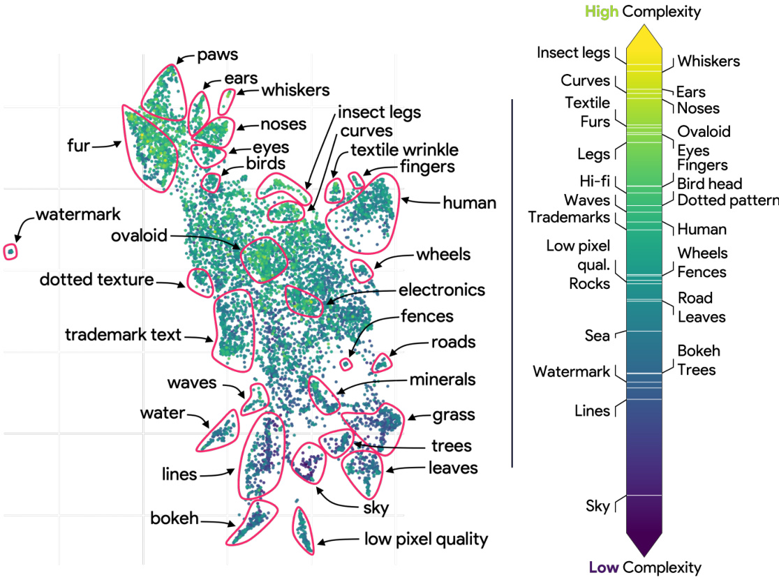
🔼 This figure shows a 2D UMAP projection of 10,000 features extracted from a ResNet50 model trained on ImageNet. These features were clustered into 150 groups (meta-features) using K-means. The left panel visualizes the meta-features, while the right panel shows the average complexity score for each meta-feature cluster. Simple features tend to be color or texture detectors, while complex features detect more structured objects or shapes.
read the caption
Figure 2: Qualitative Analysis of “Meta-feature” (cluster of features) Complexity. (Left) A 2D UMAP projection displaying the 10,000 extracted features. The features are organized into 150 clusters using K-means clustering applied to the feature dictionary D*. 30 clusters were selected for analysis of features at different complexity levels. (Right) For each Meta-feature cluster, we compute the average complexity score. This allows us to classify the features based on their complexity according to the model. Notably, simple features are often akin to color detectors (e.g., grass, sky) and detectors for low-frequency patterns (e.g., bokeh detector) or lines. In contrast, complex features encompass parts or structured objects, as well as features resembling shapes (such as ears or curve detectors). Visualizations of individual Meta-features are presented in Appendix B.

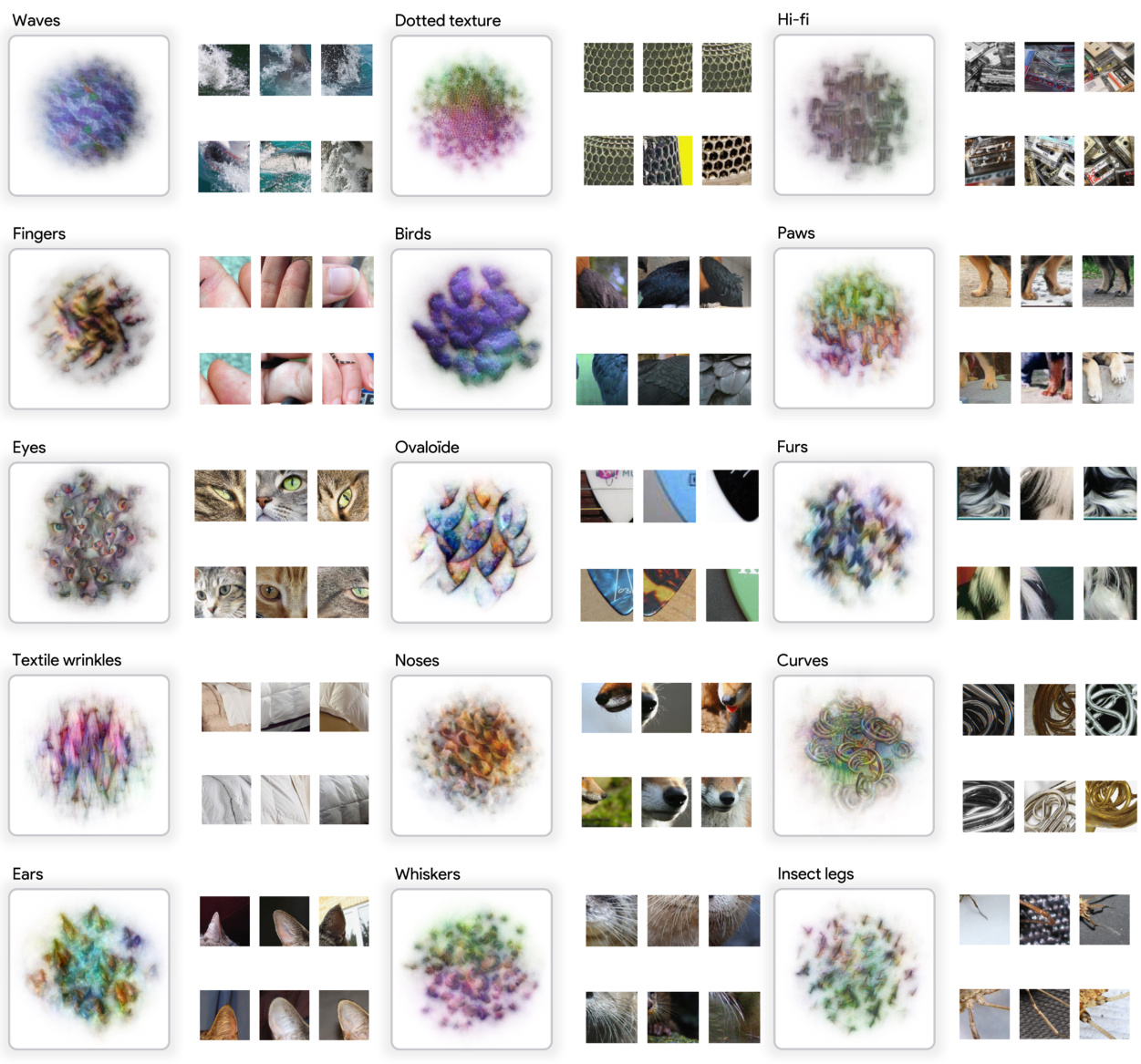
🔼 This figure visualizes meta-features (clusters of features) sorted by their complexity. Each meta-feature is represented by a composite image showing maximally activating images for that meta-feature. The figure demonstrates a progression from simple features (e.g., color, texture) to more complex features (e.g., object parts, shapes). This visualization aids in understanding the types of features learned by the model at different complexity levels.
read the caption
Figure 3: Visualization of Meta-features, sorted by Complexity. We use Feature visualization [84, 31] to visualize the Meta-features found after concept extraction. The entire visualization for each Meta-feature can be found in Appendix B.
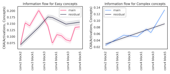
🔼 This figure shows the information flow of simple and complex features through the ResNet architecture. The left panel shows that simple features are primarily processed in the residual branches, with information transfer to later layers happening directly via residual connections. In contrast, the right panel demonstrates that for complex features, both the main and residual branches contribute to feature construction throughout the network’s layers.
read the caption
Figure 4: Simple Features Teleported by Residuals. (Left) CKA between residual branch activations fe and final concept value z. For simple concepts, beyond a certain layer (block 3), the residual already carries nearly all the information, effectively teleporting it to the last layer. (Right) Conversely, for complex features, both the main and residual branches gradually construct the features during the forward pass.
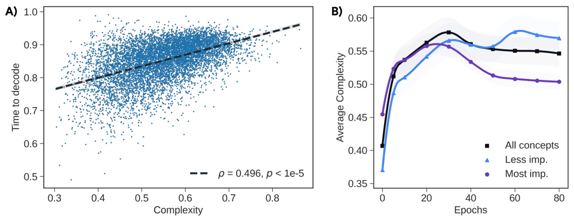
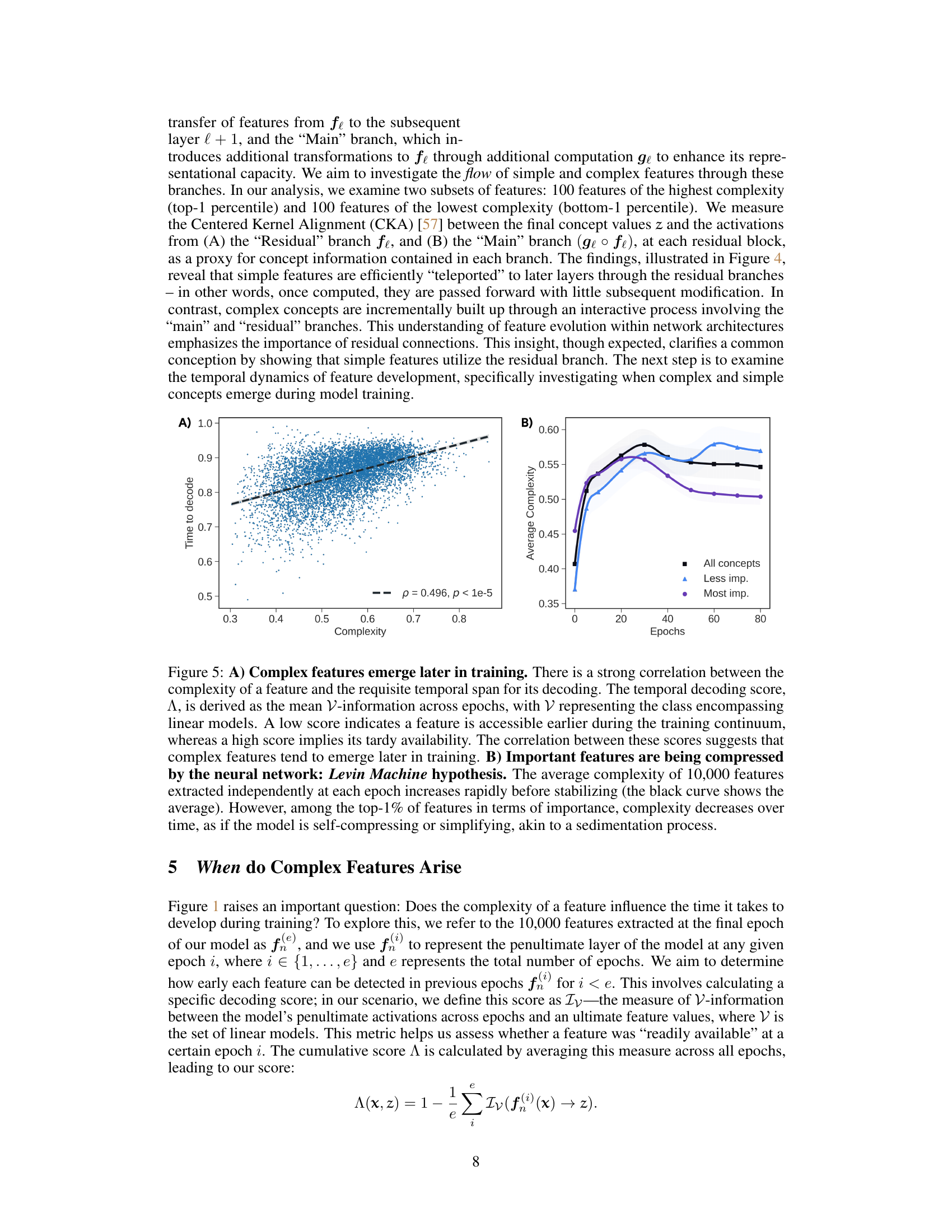
🔼 This figure shows two plots. Plot A shows a strong positive correlation between feature complexity and the time it takes for that feature to become accessible during training. Plot B shows that the average complexity of all features increases early in training and then plateaus, while the average complexity of the most important features actually decreases over time. This suggests that the model learns simpler representations for its most important features as training progresses.
read the caption
Figure 5: A) Complex features emerge later in training. There is a strong correlation between the complexity of a feature and the requisite temporal span for its decoding. The temporal decoding score, A, is derived as the mean V-information across epochs, with V representing the class encompassing linear models. A low score indicates a feature is accessible earlier during the training continuum, whereas a high score implies its tardy availability. The correlation between these scores suggests that complex features tend to emerge later in training. B) Important features are being compressed by the neural network: Levin Machine hypothesis. The average complexity of 10,000 features extracted independently at each epoch increases rapidly before stabilizing (the black curve shows the average). However, among the top-1% of features in terms of importance, complexity decreases over time, as if the model is self-compressing or simplifying, akin to a sedimentation process.

🔼 This figure shows the relationship between feature complexity and importance at two different stages of training (epoch 1 and epoch 90) in a ResNet50 model. At the beginning of training (epoch 1), there’s no clear correlation between complexity and importance. However, by the end of training (epoch 90), a strong negative correlation emerges; simpler features are more important, demonstrating the model’s preference for simpler features over time.
read the caption
Figure 6: Simplicity bias appears during training. Complexity vs. Importance of 10,000 features extracted from a ResNet50 at Epochs 1 and 90 of training. In Epoch 1, important features are not necessarily simple and seem uniformly distributed. In contrast, by the end of training, there is a clear simplicity bias, consistent with numerous studies: the model prefers to rely on simpler features.
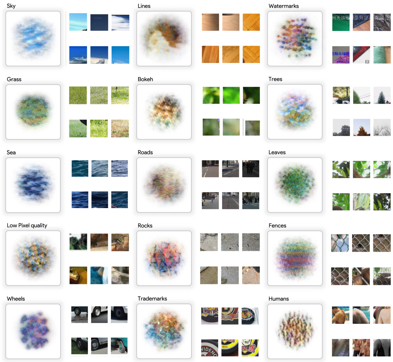
🔼 This figure displays visualizations of 15 meta-features, ordered from simplest to most complex. Each meta-feature is a cluster of similar features extracted from the penultimate layer of a ResNet50 model trained on ImageNet. The visualizations show images that maximally activate each meta-feature, illustrating the types of visual patterns each represents. Simpler meta-features tend to correspond to basic visual properties (e.g., color, texture), while more complex meta-features represent more structured object parts or shapes.
read the caption
Figure 7: Visualization of Meta-features, sorted by Complexity. Feature visualization using MACO [31] for the most simple (1-15) of the 30 Meta-features found on the 10,000 features extracted.
🔼 This figure qualitatively analyzes the complexity of features extracted from a ResNet50 model trained on ImageNet. The left panel shows a 2D UMAP projection of 10,000 features, clustered into 150 groups (meta-features) using K-means. Thirty meta-feature clusters are selected for analysis. The right panel shows the average complexity score for each meta-feature cluster, revealing a spectrum from simple (color, lines, low-frequency patterns) to complex (structured objects, shapes).
read the caption
Figure 2: Qualitative Analysis of “Meta-feature” (cluster of features) Complexity. (Left) A 2D UMAP projection displaying the 10,000 extracted features. The features are organized into 150 clusters using K-means clustering applied to the feature dictionary D*. 30 clusters were selected for analysis of features at different complexity levels. (Right) For each Meta-feature cluster, we compute the average complexity score. This allows us to classify the features based on their complexity according to the model. Notably, simple features are often akin to color detectors (e.g., grass, sky) and detectors for low-frequency patterns (e.g., bokeh detector) or lines. In contrast, complex features encompass parts or structured objects, as well as features resembling shapes (such as ears or curve detectors). Visualizations of individual Meta-features are presented in Appendix B.

🔼 The figure shows a plot of relative accuracy versus the proportion of kept concepts. The plot demonstrates that while the removal of a large number of complex features (which individually have little impact on the model’s performance) significantly reduces the model’s accuracy. This illustrates the concept of ‘support features’, a large set of complex features which individually have a small contribution, but cumulatively are essential for the model’s performance.
read the caption
Figure 9: 'Support Features' hypothesis. The majority of complex features are not very important, but play a non-negligible role and contribute to significant performance gains. This paradox is referred to as the 'support features,' a large ensemble of features individually of little to very little importance to the model but collectively holding a significant role.
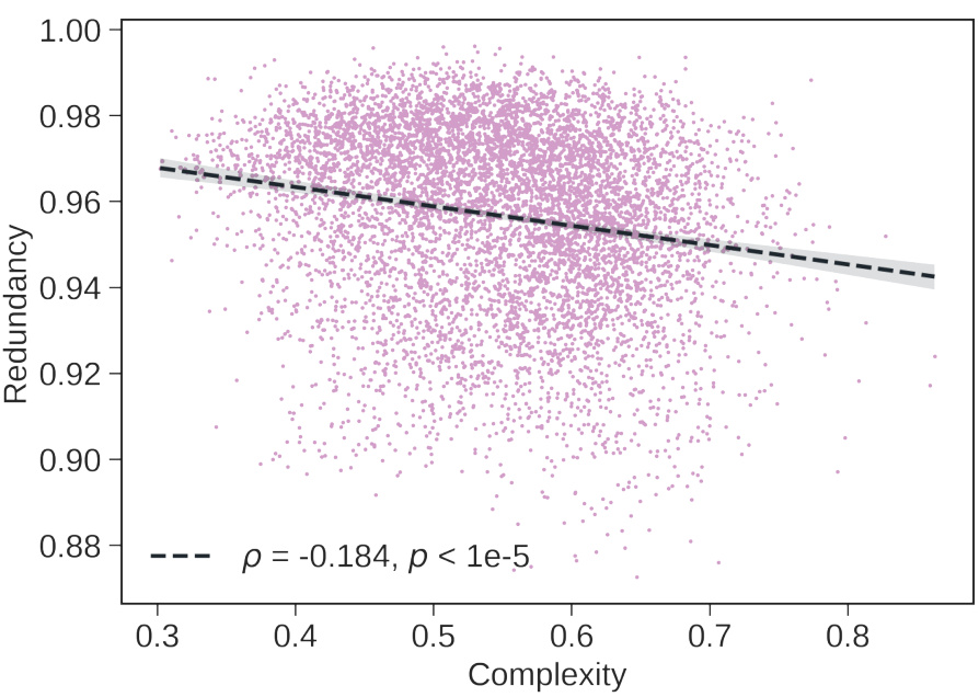
🔼 This figure shows the negative correlation between feature complexity and redundancy. The redundancy measure used quantifies how much the information of a feature is spread across multiple neurons. A low redundancy score indicates that the feature’s information is concentrated in a smaller number of neurons, while a high score suggests it’s distributed more broadly. The plot demonstrates that more complex features tend to have lower redundancy, meaning their information is more localized within the network.
read the caption
Figure 10: Complex features are less redundant. Using the redundancy measure from [76], we show that our complex features tend to be less redundant. This result also confirms a link between our complexity measure and the one recently proposed by [24], which is also based on redundancy.
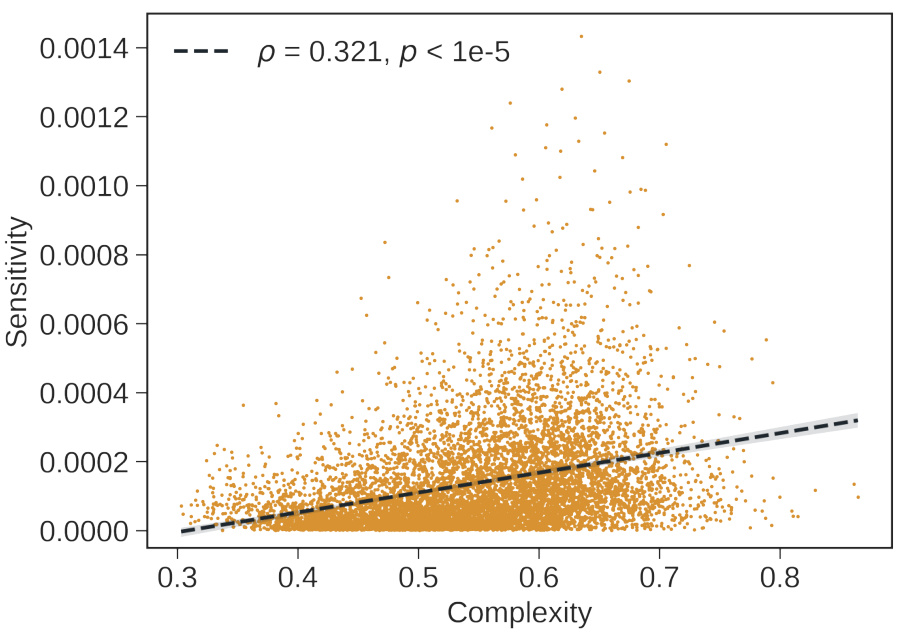
🔼 This figure shows the relationship between feature complexity and robustness. Robustness is measured by how much the feature’s value changes when Gaussian noise is added to the input image. The plot shows a negative correlation, indicating that more complex features tend to be less robust (more sensitive to noise).
read the caption
Figure 11: Complex features are less robust. This figure illustrates the relationship between feature complexity and robustness, quantified as the variance of the feature value when the image is perturbed with Gaussian noise. The results indicate that more complex features tend to exhibit lower robustness.

🔼 This figure shows the relationship between feature complexity and importance. Each point represents a feature, categorized as either ‘promoting’ (adding information to a class) or ‘inhibiting’ (removing information from a class). Violet points represent features that inhibit a class. The x-axis represents feature complexity, while the y-axis represents feature importance. The plot illustrates that important features can impact class prediction in two ways: by promoting or inhibiting.
read the caption
Figure 12: Inhibiting and non-inhibiting features vs complexity. Important features can be significant either by inhibition, i.e., removing information from a class, or by adding information for a given class. Each point represents a feature, and violet-colored features generally act as inhibitors (Γ(zi) < 0).

🔼 This figure visualizes the relationship between feature similarity and super-classes using UMAP. Each point represents a feature, colored by its superclass. The proximity of points indicates feature similarity. The clustering of features associated with certain superclasses (e.g., birds, dogs) is evident, while others are more dispersed, indicating features that are not strongly associated with a single superclass. Comparing this to Figure 2 helps determine which meta-features are ‘pure’ (one superclass) vs. ‘impure’ (multiple superclasses), revealing complexity patterns.
read the caption
Figure 13: Feature Similarity vs Super-Class. Each point represents a concept, with its color indicating the associated super-class. Some super-classes such as birds, reptiles, dogs & other mammals form well-defined, tight clusters, suggesting that features belonging to them are close in the feature space. Others, such as device, clothes appear more dispersed. By comparing this figure with Figure 2, we can identify which meta-features are 'pure' (belonging to a single super-class) and which are 'impure' (spanning multiple super-classes). Interestingly, the 'impurity' region seems to cover low-complexity and mid-complexity concepts such that Grass, Waves, Trees, Low-pixel quality detector which are not class-specific.

🔼 This figure shows the distribution of features based on their complexity, visualized using UMAP and a dendrogram. Panel A’s UMAP plot shows that features cluster in distinct regions of varying complexity. Panel B’s dendrogram further supports this, showing a clear separation of features by complexity at each hierarchical level. Simpler features cluster together, as do more complex features. This suggests that feature complexity is a meaningful organizational principle within the model.
read the caption
Figure 14: Feature Similarity by Complexity. A) Each point is a feature, colored by its complexity score. Distinct areas of the graph correspond to varying levels of complexity, suggesting a non-random distribution of feature complexity. For instance, animal-related features tend to have higher complexity, one could hypothesize that the fine-grained classification required for these categories are responsible for this complexity. B) A four-level dendrogram where each level further segments clusters and calculates the average complexity for each sub-cluster. A clear split by complexity appears at the first level and intensifies with depth, supporting the idea that some regions of the feature space are inherently more complex than others.

🔼 This figure shows how features are clustered based on their importance. Panel A uses UMAP to visualize the features, where each point’s color represents its importance score. More important features cluster at the top of the graph. Panel B shows a dendrogram of four levels, showing how feature clusters are divided based on their average importance. The top level of the dendrogram shows a clear separation between high and low-importance feature groups. The results suggest there’s a relationship between feature importance and their spatial arrangement in the feature space.
read the caption
Figure 15: Feature Similarity by Importance. A) Each point represents a feature, with color indicating its importance. Distinct regions of the graph contain features of varying importance, particularly with more important features clustering at the top. B) A four-level dendrogram with sub-clusters evaluated by their average importance. We observe that from the first level, the dendrogram effectively splits features into groups of varying importance, corresponding to the upper and lower parts of the UMAP graph in Panel A.
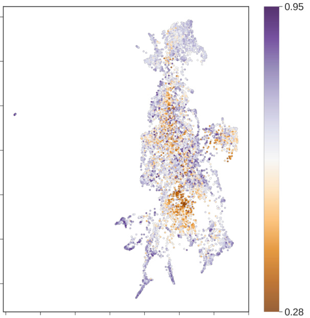
🔼 This figure visualizes the distribution of 10,000 features extracted from a ResNet50 model based on their Hoyer scores. The Hoyer score quantifies the degree of localization or distribution of a feature across neurons. A higher score indicates a feature primarily encoded by a single neuron (’local’), while a lower score indicates the feature is distributed across many neurons (‘distributed’). The color of each point in the UMAP embedding represents the Hoyer score, showing a range from highly local to highly distributed encoding strategies.
read the caption
Figure 16: Local vs Distributed Encoding. Each point represents a feature, with color indicating its Hoyer score. Higher scores suggest a more 'local' representation, where a feature is primarily encoded by a single neuron. Lower scores indicate a distributed representation across a population of neurons. Interestingly, some features have scores near 1, implying near-complete localization, while others are more distributed. This variation highlights the diversity in encoding across features.

🔼 This figure displays a scatter plot showing the relationship between feature complexity and the Hoyer score, a measure of how distributed the encoding of a feature is across neurons. A linear regression is also shown. The results suggest there is no significant correlation between the two variables, indicating that feature complexity does not strongly influence whether a feature is encoded locally or distributedly.
read the caption
Figure 17: Feature Complexity vs. Distributed Encoding. We show that there is no clear relationship between feature complexity and the degree of distributed encoding. Whether a feature is encoded by a single neuron or distributed across multiple neurons does not seems to be determined by its complexity.

🔼 This figure shows how simple and complex features flow through a ResNet50. Simple features largely use the residual connections, bypassing much of the visual hierarchy. In contrast, complex features are gradually constructed through interactions between the main branch and the residual connections, requiring more processing steps.
read the caption
Figure 4: Simple Features Teleported by Residuals. (Left) CKA between residual branch activations fe and final concept value z. For simple concepts, beyond a certain layer (block 3), the residual already carries nearly all the information, effectively teleporting it to the last layer. (Right) Conversely, for complex features, both the main and residual branches gradually construct the features during the forward pass.
Full paper#

