TL;DR#
Deep learning often exhibits unpredictable behavior, hindering our understanding of its inner workings and optimal design choices. Existing methods for analyzing neural networks, such as those based on tangent kernels, often fail to capture the dynamic complexities during training. This lack of understanding poses significant challenges for advancing deep learning research and engineering robust models.
This paper introduces a new “telescoping model” to overcome these issues. By incrementally approximating neural network training as a sequence of first-order updates, the model provides a clearer and more accurate representation of the entire learning process. Using this model, the researchers gained new empirical insights into double descent, grokking, and gradient boosting, revealing unexpected connections between these phenomena and offering valuable insights for improved model design and optimization.
Key Takeaways#
Why does it matter?#
This paper is crucial for researchers in deep learning due to its novel approach to understanding neural networks’ behavior. It offers new empirical insights into complex phenomena and provides a pedagogical framework for analyzing training processes, which could significantly impact future research on model design and optimization. The study also reveals surprising parallels between deep learning and gradient boosting, potentially inspiring innovative hybrid approaches.
Visual Insights#

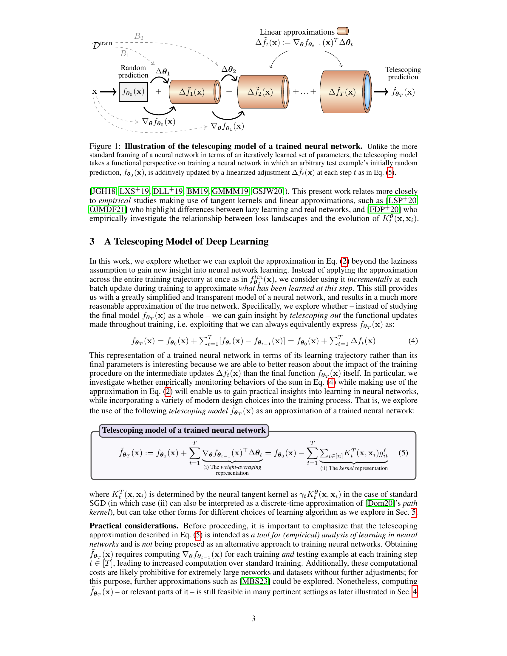
🔼 This figure illustrates the telescoping model of deep learning. It shows how a neural network’s prediction for a given input starts randomly and is iteratively refined through additive updates (Aft(x)). Each update is a linear approximation of the change in prediction based on the gradient of the loss function with respect to the parameters. The final prediction (f~θT(x)) is the sum of the initial prediction and all these incremental linear adjustments, offering a functional view of the training process, unlike traditional parameter-centric models. This process is visually represented by a sequence of cylinders, each representing a training step.
read the caption
Figure 1: Illustration of the telescoping model of a trained neural network. Unlike the more standard framing of a neural network in terms of an iteratively learned set of parameters, the telescoping model takes a functional perspective on training a neural network in which an arbitrary test example's initially random prediction, fe (x), is additively updated by a linearized adjustment A ft (x) at each step t as in Eq. (5).

🔼 This figure compares the approximation error of two models: the telescoping model and a linear model linearized around initialization. It shows that iteratively using the telescoping model significantly improves the approximation compared to using just the linear model. The improvement is substantial, especially in later optimization steps.
read the caption
Figure 7: Approximation error of the telescoping (fo₁ (x), red) and the model linearized around the initialization (foin(x), gray) by optimization step for different optimization strategies and other design choices. Iteratively telescoping out the updates using fe, (x) improves upon the lazy approximation around the initialization by orders of magnitude.
In-depth insights#
Telescoping Lens Model#
The proposed “Telescoping Lens Model” offers a novel way to analyze neural network training. Instead of focusing solely on the final network parameters, it incrementally tracks the functional changes made at each training step. This approach allows for a more granular understanding of the learning process, revealing insights into phenomena like double descent and grokking that are not readily apparent through traditional methods. By linearly approximating the functional updates, the model provides a simplified but informative lens to examine the behavior of complex networks. The use of this telescoping method makes it possible to isolate the effects of various design choices (architecture, optimization strategy), thereby facilitating better model understanding. Crucially, it also allows for the creation of novel metrics to evaluate model complexity, furthering the understanding of generalization capabilities. The model’s simplicity also makes it suitable for pedagogical applications. Overall, the “Telescoping Lens Model” presents a powerful tool for both empirical and theoretical investigation of neural network training dynamics.
Empirical Analyses#
An empirical analysis section in a research paper would ideally present a robust and detailed examination of experimental results. It should go beyond simply stating findings and delve into a thorough interpretation of the data, addressing potential biases or limitations. Statistical significance testing would be crucial, employing appropriate metrics to determine the reliability of observations. The analysis should demonstrate a clear understanding of the relationships between variables and provide visualizations that effectively communicate complex patterns. Comparison of various model architectures or hyperparameter settings would show a comprehensive investigation. Importantly, the section should directly support the paper’s main claims, providing strong evidence and linking observed phenomena to theoretical background. A thoughtful discussion of unexpected results or deviations from expectations also shows rigor and strengthens the overall contribution of the paper.
GBT vs Neural Nets#
The comparison between Gradient Boosting Trees (GBTs) and neural networks reveals interesting strengths and weaknesses of each approach. GBTs often outperform neural networks on tabular data, particularly when dealing with datasets containing irregularities or heterogeneous features, likely due to the different inductive biases and kernel functions employed by each. Neural networks excel in domains with abundant, homogeneous data like images and text. GBTs’ tree-based structure leads to more predictable generalization behavior, especially in the presence of unusual test inputs, unlike the sometimes unpredictable nature of neural network tangent kernels which can change significantly during training. The telescoping model provides a valuable lens for understanding these differences, offering a clearer way to directly compare the incremental training processes and functional changes in both paradigms. By isolating components of each algorithm’s learning trajectory, the analysis could unlock strategies to improve neural network performance on tabular datasets or to leverage the interpretability of GBTs for increased transparency in neural network training.
Weight Averaging#
Weight averaging in deep learning is a surprising phenomenon where averaging the weights of two independently trained neural networks can yield a model that performs comparably to, or even better than, the individual networks. This contrasts with the typical intuition that averaging the highly nonlinear functions represented by the weights would likely degrade performance. The success of weight averaging is particularly noteworthy in scenarios where linear mode connectivity (LMC) exists, meaning the solution space allows for simple linear interpolation between different solutions. The paper investigates how the model’s gradient stabilization during training relates to the emergence of LMC and weight averaging success. This is particularly important in complex optimization landscapes, where weight averaging can help overcome the challenges of reaching optimal solutions. While the paper suggests that consistent gradient behavior contributes to successful weight averaging, it also notes that additional factors like dataset properties and architectural design choices play a role, indicating that further research is needed for a complete understanding of this phenomenon. The paper uses a ’telescoping lens’ approach to shed light on this behavior empirically, suggesting the framework as a promising avenue for further research into weight averaging in deep learning.
Design Choice Effects#
The section on ‘Design Choice Effects’ would explore how various design decisions made during the development of a deep learning model impact its performance and characteristics. It would likely delve into the effects of different optimization algorithms (e.g., SGD, Adam, AdamW), analyzing how these choices influence the model’s convergence speed, generalization ability, and sensitivity to hyperparameters. Key findings might showcase how momentum or weight decay significantly alter the training dynamics, affecting the model’s generalization curve and resilience to overfitting. Furthermore, the impact of different activation functions (e.g., ReLU, sigmoid, tanh) on the model’s capacity to learn complex patterns and its behavior in various scenarios would be examined. The analysis would also likely encompass the consequences of architectural choices, specifically the number of layers, the width of layers (number of neurons per layer), the choice of layers (e.g. convolutional vs. fully connected), and regularization techniques employed (e.g., dropout, batch normalization). The study would aim to provide a nuanced understanding of how these design parameters interact, uncovering potential synergies or tradeoffs that can guide the design of efficient and effective deep learning models. Crucially, the findings could offer valuable insights into overcoming common challenges like double descent or grokking, potentially proposing novel design strategies to improve model robustness and performance in such complex scenarios.
More visual insights#
More on figures
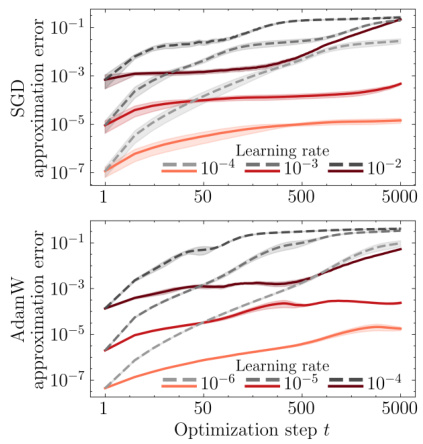
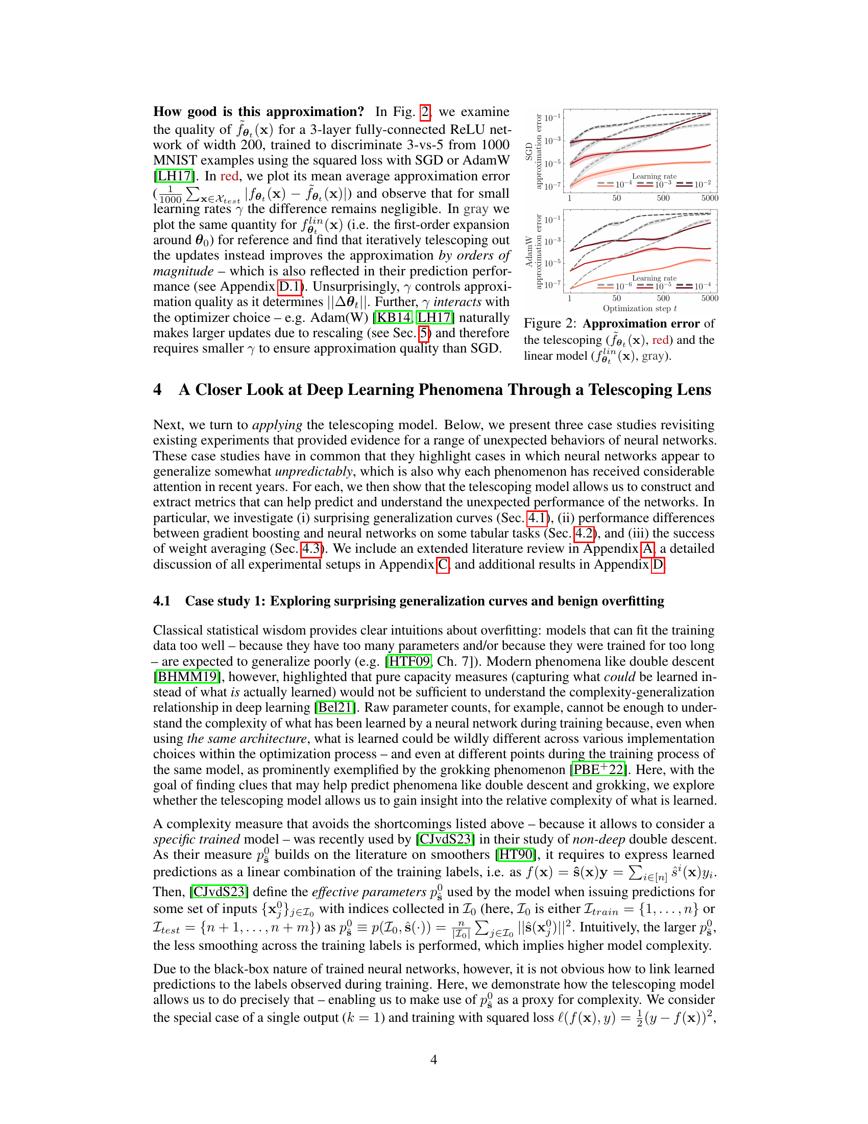
🔼 This figure compares the approximation errors of two models: the telescoping model (fo₁ (x)) and a linear model (foin (x)). The telescoping model is an iterative approximation of a trained neural network, while the linear model is a first-order approximation around the initialization point. The plot shows that using smaller learning rates reduces the approximation errors for both models. However, the telescoping model consistently yields a much better approximation than the linear model. The optimizer used also affects approximation quality; AdamW (KB14, LH17), which naturally makes larger updates due to rescaling, necessitates smaller learning rates to obtain the same approximation quality as SGD.
read the caption
Figure 2: Approximation error of the telescoping (fo₁ (x), red) and the linear model (foin (x), gray).
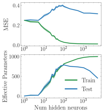
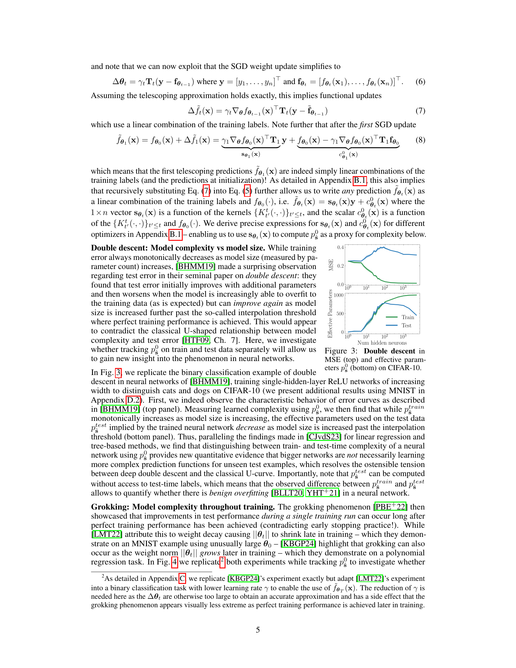
🔼 This figure shows the results of a double descent experiment on the CIFAR-10 dataset. The top panel displays the mean squared error (MSE) on both the training and testing sets as a function of the number of hidden neurons in a single-hidden-layer ReLU network. The bottom panel shows the corresponding effective parameters (p) calculated using the telescoping model, separately for the training and testing sets. The figure illustrates the non-monotonic relationship between model size and test error that is characteristic of double descent, and demonstrates how the telescoping model’s complexity metric can quantify this phenomenon by tracking the divergence between training and test complexity.
read the caption
Figure 3: Double descent in MSE (top) and effective parameters p (bottom) on CIFAR-10.
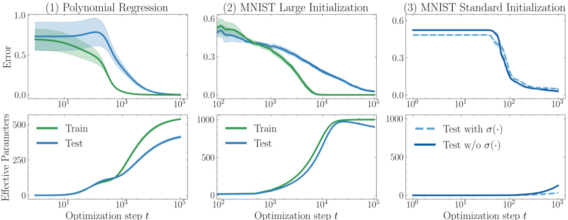
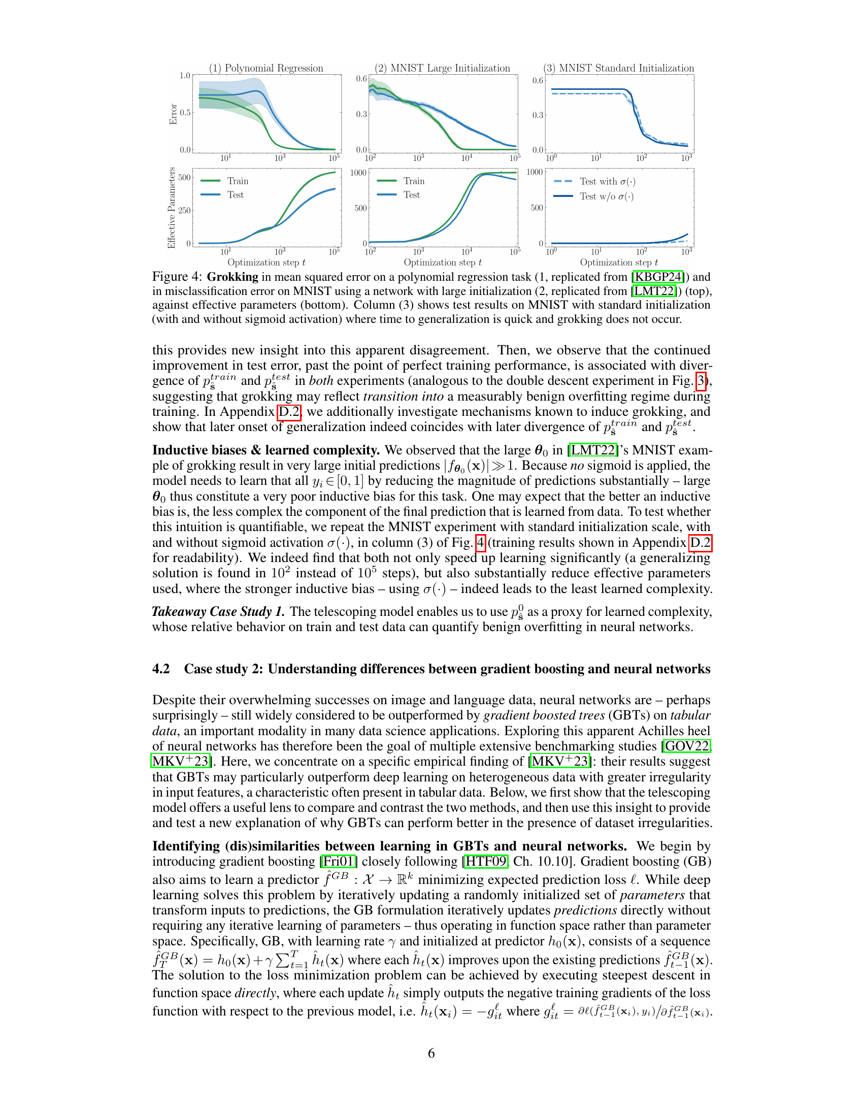
🔼 This figure displays the results of three grokking experiments. The top row shows the mean squared error (MSE) for a polynomial regression task and the misclassification error for MNIST datasets with large and standard initializations. The bottom row shows the corresponding effective parameters (p) for each case. The experiments highlight the relationship between grokking, model complexity, and different initialization strategies. The use of a sigmoid activation function is also explored in one of the MNIST experiments, which influences the learning dynamics and complexity.
read the caption
Figure 4: Grokking in mean squared error on a polynomial regression task (1, replicated from [KBGP24]) and in misclassification error on MNIST using a network with large initialization (2, replicated from [LMT22]) (top), against effective parameters (bottom). Column (3) shows test results on MNIST with standard initialization (with and without sigmoid activation) where time to generalization is quick and grokking does not occur.
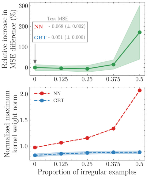
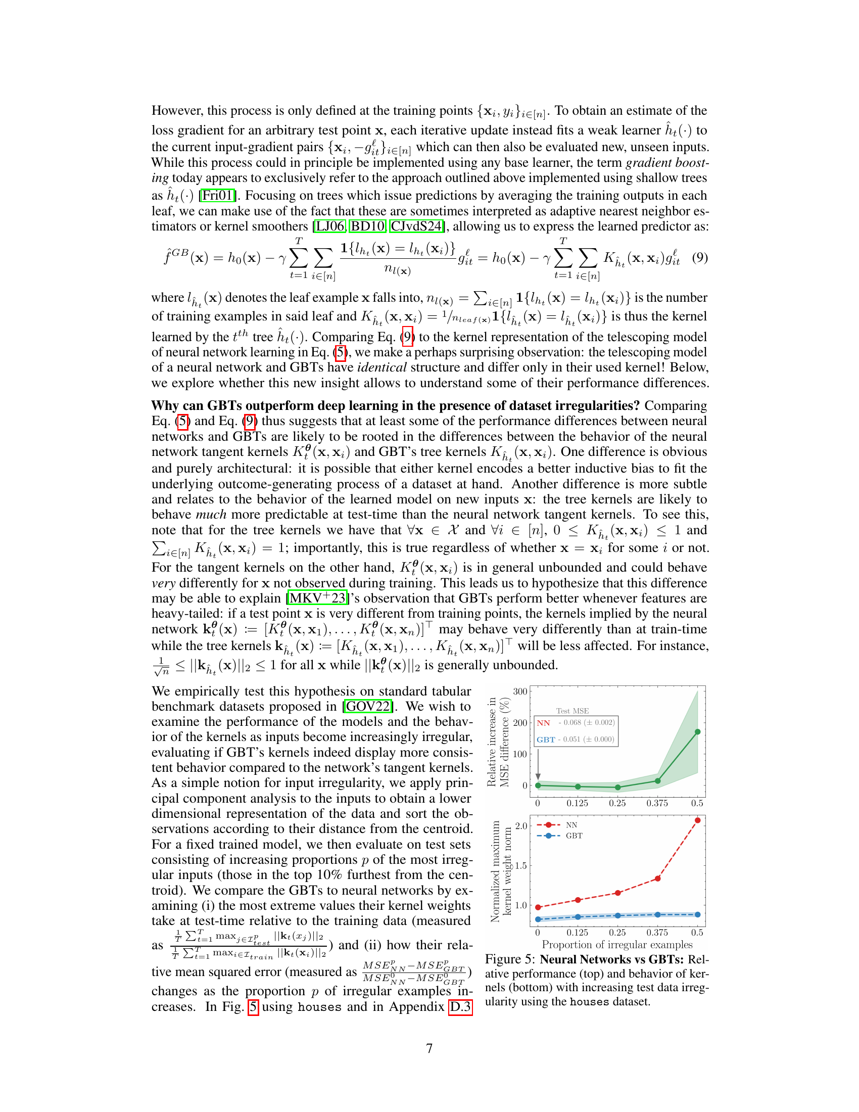
🔼 This figure compares the performance of neural networks and gradient boosted trees (GBTs) on the ‘houses’ dataset as the proportion of irregular examples in the test set increases. The top panel shows the relative increase in mean squared error (MSE) difference between the two models. The bottom panel shows the normalized maximum kernel weight norm for both models. This visualization helps illustrate how the behavior of the models’ kernels contributes to their performance differences, particularly in scenarios with more irregular data.
read the caption
Figure 5: Neural Networks vs GBTs: Relative performance (top) and behavior of kernels (bottom) with increasing test data irregularity using the houses dataset.

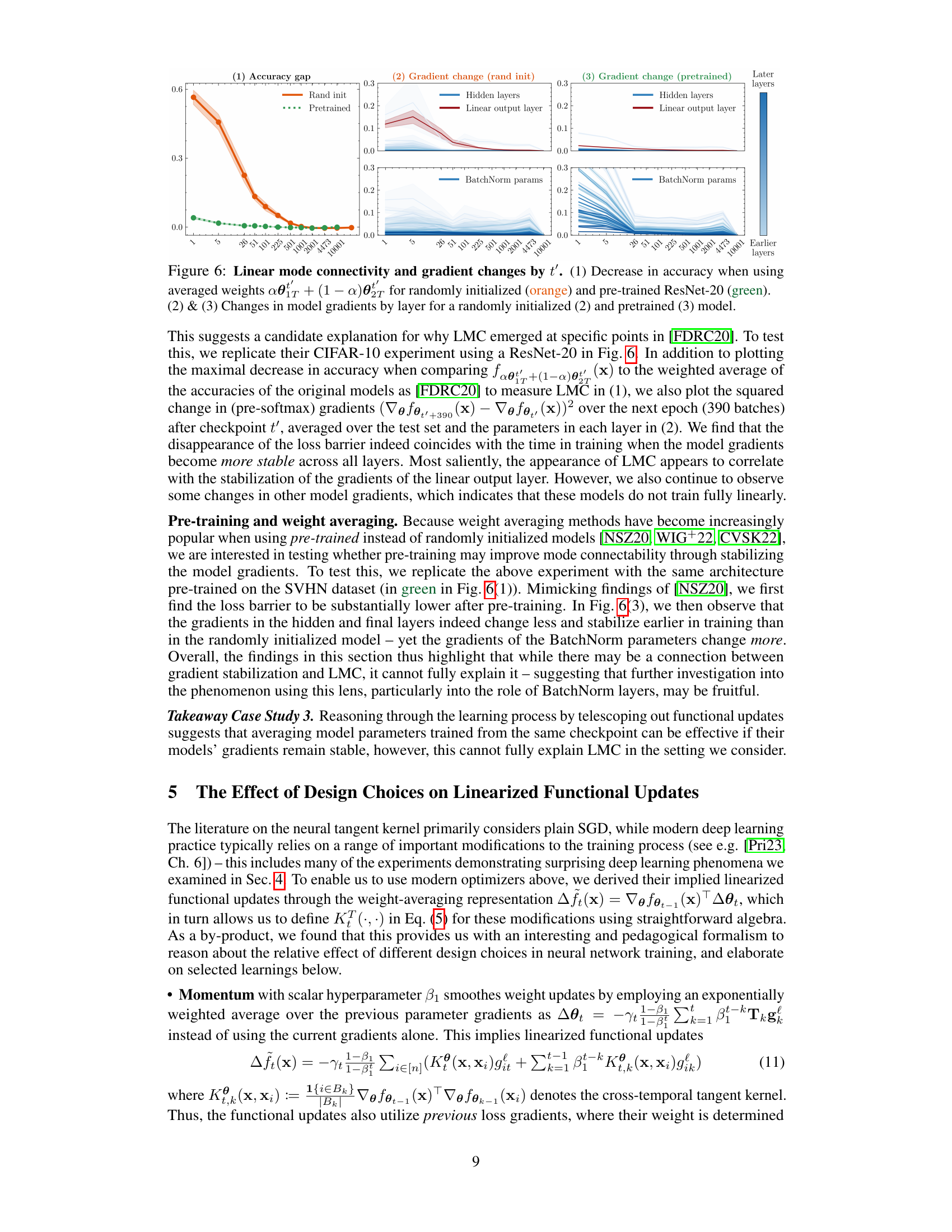
🔼 This figure shows the results of an experiment investigating linear mode connectivity (LMC) and how it relates to gradient stabilization. The experiment uses a ResNet-20 model, comparing randomly initialized and pre-trained versions. Panel (1) shows the decrease in accuracy when averaging weights at different checkpoints during training. Panels (2) and (3) show the change in model gradients across layers for both randomly initialized and pre-trained models. The results suggest that gradient stabilization correlates with LMC.
read the caption
Figure 6: Linear mode connectivity and gradient changes by t'. (1) Decrease in accuracy when using averaged weights αθτ + (1 − a) for randomly initialized (orange) and pre-trained ResNet-20 (green). (2) & (3) Changes in model gradients by layer for a randomly initialized (2) and pretrained (3) model.

🔼 This figure shows the approximation error of two models: the telescoping model and a simple linear model. The x-axis represents the learning rate, and the y-axis represents the approximation error. The figure shows that for small learning rates, the error of the telescoping model is negligible. This suggests that the telescoping model is a good approximation of the true neural network for small learning rates. The figure also shows that the telescoping model is a better approximation than the linear model, especially for larger learning rates. The different colored lines represent different optimizers used.
read the caption
Figure 2: Approximation error of the telescoping (fo₁ (x), red) and the linear model (foin (x), gray).
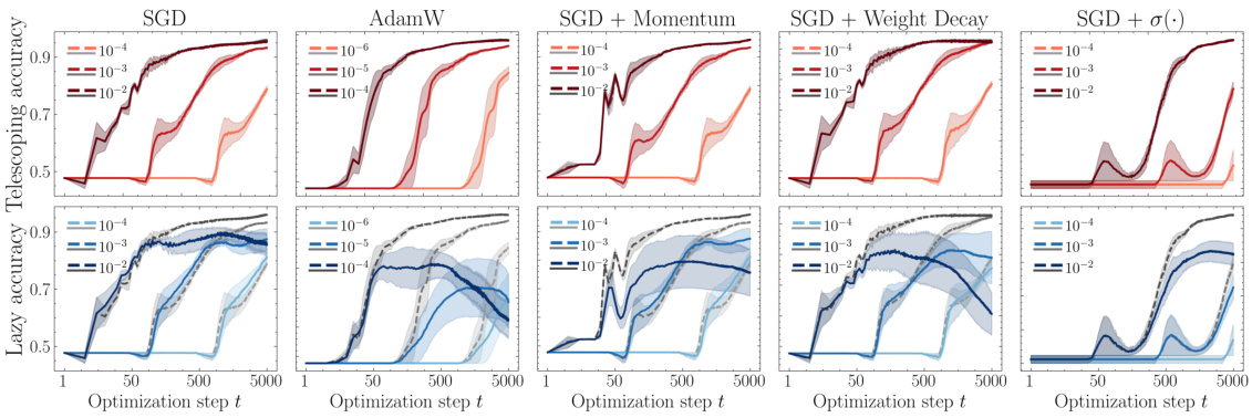
🔼 This figure compares the accuracy of three different models over the course of training: the telescoping model, a linear approximation, and the actual neural network. It demonstrates that the telescoping model closely tracks the accuracy of the real neural network, while the linear approximation significantly diverges as training progresses, highlighting the accuracy and utility of the telescoping model for analyzing deep learning phenomena.
read the caption
Figure 8: Test accuracy of the telescoping (fo₁ (x), red, top row) and the model linearized around the initialization (foin(x), blue, bottom row) against accuracy of the actual neural network (gray) by optimization step for different optimization strategies and other design choices. While the telescoping model visibly matches the accuracy of the actual neural network, the linear approximation around the initialization leads to substantial differences in accuracy later in training.
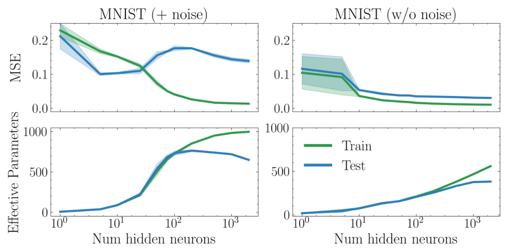
🔼 This figure shows the results of double descent experiments on the MNIST dataset. The left panel displays the results when 20% label noise is added during training, while the right panel shows the results without added noise. The x-axis represents the number of hidden neurons in the model, and the y-axis shows the mean squared error (MSE). The key observation is that the characteristic double descent curve (initial improvement, then a dip, then another rise) only emerges when label noise is present. Without noise, test error decreases monotonically with increased model size.
read the caption
Figure 9: Double descent experiments using MNIST, distinguishing 3-vs-5, with 20% added label noise during training (left) and no added label noise (right). Without label noise, there is no double descent in error on this task; when label noise is added we observe the prototypical double descent shape in test error.
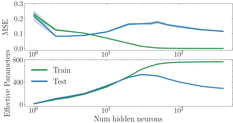
🔼 This figure shows the double descent phenomenon observed in a neural network trained on the CIFAR-10 dataset. The top panel displays the mean squared error (MSE) on the test set as a function of the number of hidden neurons in a single-hidden-layer ReLU network. The bottom panel shows the effective number of parameters (p) used by the model, calculated using a new metric introduced in the paper, as a function of the number of hidden neurons. The plot demonstrates that test error initially decreases with increasing model size, then increases (overfitting), and finally decreases again as the model size significantly surpasses the amount of training data, exhibiting the double descent phenomenon. The effective parameters on the training set monotonically increase with model size, while test-time effective parameters show non-monotonic behavior, decreasing beyond the interpolation threshold. This divergence in effective parameters between training and test sets is linked to the non-monotonic generalization curve.
read the caption
Figure 3: Double descent in MSE (top) and effective parameters p (bottom) on CIFAR-10.
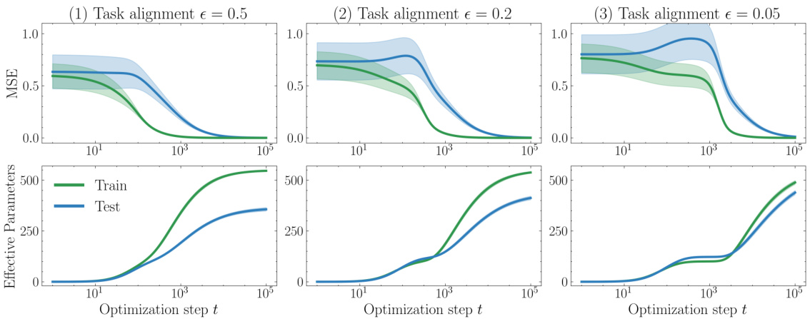
🔼 This figure shows the results of a polynomial regression experiment. The top panels show mean squared error (MSE) over optimization steps for three different levels of task alignment (epsilon). The bottom panels display the effective number of parameters used during training (green) and testing (blue) for the same three task alignment levels. The plots illustrate the grokking phenomenon, where improvements in test performance occur after perfect training performance is already achieved.
read the caption
Figure 11: Grokking in mean squared error (top) on a polynomial regression task (replicated from [KBGP24]) against effective parameters (bottom) with different task alignment parameters €.
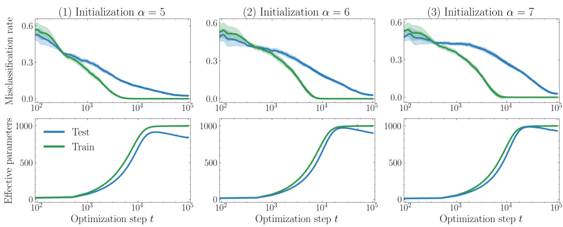
🔼 This figure shows the results of replicating an experiment from the paper [LMT22] on the MNIST dataset. Three experiments are shown, each with a different initialization scale (‘a’). The top row displays the misclassification error (test and train) over training steps. The bottom row shows the effective number of parameters (test and train) over training steps. The results illustrate the grokking phenomenon, where test performance improves significantly after training accuracy reaches near perfect.
read the caption
Figure 12: Grokking in misclassification error on MNIST using a network with large initialization (replicated from [LMT22]) (top), against effective parameters (bottom) with different initialization scales a.
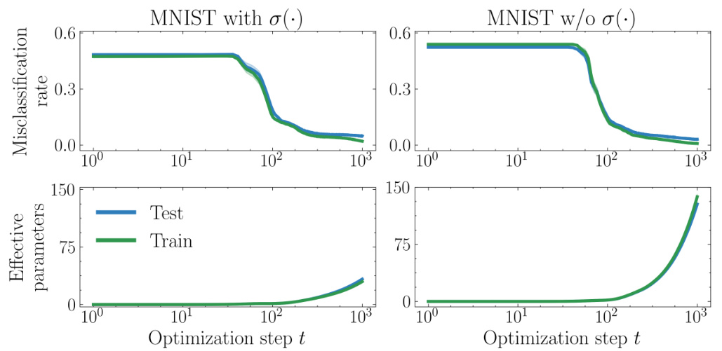
🔼 This figure displays the results of an experiment testing for the grokking phenomenon on MNIST using a network with standard initialization and comparing the results with and without using a sigmoid activation function. The top panel shows the misclassification error on the MNIST dataset, and the bottom panel shows the number of effective parameters used. The results show no grokking, with both train and test error decreasing smoothly and almost identically during training. The low number of effective parameters supports the absence of grokking. The experiment highlights the role of initialization and activation functions in influencing the learning dynamics and generalization behavior.
read the caption
Figure 13: No grokking in misclassification error on MNIST (top), against effective parameters (bottom) using a network with standard initialization (a = 1) with and without sigmoid activation.

🔼 This figure compares the performance of neural networks and gradient boosted trees (GBTs) on three additional tabular datasets from the work of [GOV22] as the proportion of irregular test examples increases. The top row shows the relative increase in the mean squared error (MSE) difference between neural networks and GBTs. The bottom row displays the normalized maximum kernel weight norm for both neural networks and GBTs. The figure demonstrates how the performance gap between the two models changes with increasing data irregularity, and how that change relates to the behavior of their respective kernels.
read the caption
Figure 14: Neural Networks vs GBTs: Relative performance (top) and behavior of kernels (bottom) with increasing test data irregularity for three additional datasets.
Full paper#
