On the Impacts of the Random Initialization in the Neural Tangent Kernel Theory

↗ OpenReview ↗ NeurIPS Homepage ↗ Chat

TL;DR

#

Key Takeaways

#

Why does it matter?

#

This paper is crucial because it challenges the widely used assumption of zero initialization in Neural Tangent Kernel (NTK) theory, which is inconsistent with real-world applications. The findings highlight the limitations of NTK theory in explaining neural network performance and open avenues for more realistic theoretical frameworks.

Visual Insights

#

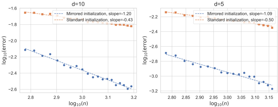
This figure compares the generalization error decay curves for networks trained with mirrored and standard initializations. Two separate plots show results for datasets with 5 and 10 dimensions, respectively. Each plot displays the logarithm of the generalization error (y-axis) against the logarithm of the number of samples (x-axis). The data points represent the average error over 20 trials. Linear regression lines highlight the different slopes of error decay under the two initialization methods, demonstrating a steeper decline for mirrored initialization.

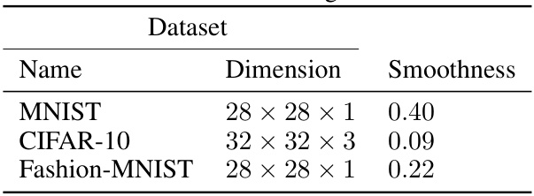
This table presents the smoothness of the goal function for three image datasets: MNIST, CIFAR-10, and Fashion-MNIST. The smoothness values (0.40, 0.09, and 0.22 respectively) are calculated using a one-hidden layer neural tangent kernel (NTK) and provide insight into the complexity of the underlying regression functions. This information is crucial in the context of the paper’s analysis regarding the impact of initialization on the generalization ability of neural networks.

In-depth insights

#

NTK Initialization Impact

#

The Neural Tangent Kernel (NTK) theory, while elegant in its simplicity, relies heavily on specific initialization schemes, often employing a mirrored initialization to ensure the network’s output is zero at initialization. This paper delves into the impact of deviating from this idealized setup by exploring the effects of standard, non-zero random initialization. The key finding is that standard initialization leads to a significant performance degradation in wide neural networks, as the generalization error does not improve as efficiently as it does with mirrored initialization. This is due to the poor smoothness of the Gaussian process that the network converges to under standard initialization, leading to a slower convergence rate. This result directly challenges the typical NTK assumption and suggests that the NTK framework may not fully capture the superior generalization capabilities of neural networks, particularly those using non-mirrored initializations. Further research is needed to address this divergence and improve the accuracy of NTK theory in predicting real-world neural network behavior.

Generalization Error Bounds

#

The section on ‘Generalization Error Bounds’ would ideally delve into the theoretical guarantees of a model’s performance on unseen data. A strong analysis would establish upper bounds, defining the maximum possible error, and lower bounds, setting a minimum level of error regardless of the model’s sophistication. The key is to show how these bounds scale with factors like dataset size (n), model complexity (e.g., number of parameters), and data dimensionality (d). A well-written section would rigorously prove these bounds, highlighting the dependence on crucial assumptions like the smoothness of the target function or the noise distribution. Tight bounds, where the upper and lower limits converge, offer the most informative insights. However, even loose bounds can be valuable, especially if they reveal the model’s inherent limitations—for example, a lower bound that scales poorly with dimensionality would suggest a model’s vulnerability to the ‘curse of dimensionality’. The discussion should acknowledge any limitations or strong assumptions needed to establish the bounds, transparently addressing potential gaps between theoretical results and practical performance. Finally, the implications of the derived bounds for model selection and algorithm design should be clearly stated.

Smoothness Analysis

#

A smoothness analysis within a machine learning context often investigates the complexity of functions, particularly the relationship between a function’s smoothness and its generalization performance. Smooth functions, those that are continuous and have continuous derivatives, tend to generalize well, as they can adapt well to unseen data. Conversely, rough or discontinuous functions may overfit to training data and perform poorly on unseen examples. Analyzing smoothness can involve studying the function’s derivatives, using techniques like Sobolev spaces, which provide a quantitative measure of smoothness. Understanding the smoothness properties of neural networks is crucial, as these properties influence the network’s ability to learn and generalize. The analysis might also consider various activation functions, network architectures, and training methods, and their effects on a neural network’s smoothness. Measuring the smoothness of the target function, the underlying function that the neural network is attempting to approximate, is another important aspect. The match or mismatch between the network’s representational capacity and the target function’s complexity determines the generalization behavior.

Limitations of NTK

#

The Neural Tangent Kernel (NTK) theory, while offering valuable insights into the behavior of wide neural networks, presents certain limitations. The assumption of infinite width is unrealistic, as real-world networks have finite dimensions. This discrepancy between theoretical and practical settings significantly impacts the theory’s applicability. The reliance on gradient flow dynamics, often a simplification of actual training algorithms (like stochastic gradient descent), limits the theory’s predictive power in scenarios with non-convex landscapes and noisy data. Moreover, NTK’s success in capturing the generalization performance of networks is context-dependent. It may not fully explain the superior performance of neural networks in various tasks, particularly those that leverage implicit biases or benefit from architectural features not explicitly modeled within the NTK framework. The impact of initialization schemes also poses a challenge, as standard, non-zero initializations can deviate from the idealized zero-initialization assumptions inherent in most NTK analyses, highlighting a gap between theoretical assumptions and practical implementation. Consequently, the NTK framework should be viewed as a valuable approximation but not a complete explanation for the success of neural networks, requiring further advancements to bridge this gap between theory and practice.

Future Research

#

Future research directions stemming from this work on random initialization in Neural Tangent Kernel (NTK) theory could explore mitigating the negative impacts of standard initialization. This might involve developing new initialization schemes that balance the benefits of random exploration with improved generalization. A deeper investigation into the interaction between initialization and network architecture is also warranted, potentially revealing optimal initialization strategies for specific network types or tasks. Furthermore, extending the analysis beyond fully-connected networks to convolutional or recurrent architectures would significantly broaden the applicability of the findings. Finally, a comprehensive study comparing the theoretical predictions of NTK theory with the empirical performance of neural networks in practice is crucial for assessing the theory’s limitations and guiding future improvements. This includes examining scenarios with non-standard activation functions, data distributions, and training algorithms. Ultimately, bridging the gap between theoretical understanding and practical applications remains a key challenge.

More visual insights

#

More on figures

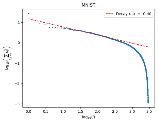
This figure displays the decay curve of the logarithm of the sum of squared coefficients for the MNIST dataset. The x-axis represents the logarithm of the index i, and the y-axis represents the logarithm of the sum of squared coefficients from index i to n (where n is the total number of samples, 3000 in this case). The blue dots show the actual data points, and the red dashed line represents a least-squares regression fit to these points, with the slope of the line indicating the decay rate (-0.40 in this case). The figure visually demonstrates the decay of coefficients, illustrating how the contribution of each component decreases as i increases, which is related to the smoothness of the goal function.

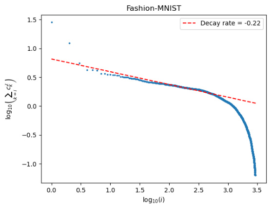
This figure shows the decay curve of the logarithm of the sum of squared coefficients for the Fashion-MNIST dataset. The x-axis represents the logarithm of the index i, and the y-axis represents the logarithm of the sum of squared coefficients from index i to n (3000 in this case). The dashed red line is a linear regression fit to the data points, and its slope represents the estimated smoothness of the function. The figure visually demonstrates the decay rate of the coefficients, which is related to the smoothness of the underlying function.

This figure displays the decay curve of the logarithm of the sum of squared coefficients for the MNIST dataset. The x-axis represents the logarithm of the index i, and the y-axis represents the logarithm of the sum of squared coefficients from i to n (where n is the total number of samples). A least-squares regression line is fitted to the data points to estimate the decay rate, which provides an approximation of the smoothness of the underlying function. The figure visually demonstrates the relationship between the index i and the magnitude of the squared coefficients, illustrating how the coefficients decay as the index increases.

Full paper

#