TL;DR#
Offline reinforcement learning faces a major challenge: overestimating the value of actions outside the training data’s distribution (OOD actions). This leads to learning policies that favor risky, poorly understood actions, ultimately resulting in poor performance. Existing methods often try to address this by making pessimistic adjustments to all Q-values, but this can be overly cautious and limit performance.
This paper introduces Q-Distribution Guided Q-Learning (QDQ), which cleverly tackles this issue. Instead of pessimistically adjusting all values, QDQ uses a consistency model to precisely estimate the uncertainty of each Q-value. It then applies a pessimistic adjustment only to the high-uncertainty Q-values (likely corresponding to OOD actions). Further, an uncertainty-aware optimization objective ensures the algorithm doesn’t become excessively cautious. The results show that QDQ significantly outperforms existing methods on several benchmark datasets.
Key Takeaways#
Why does it matter?#
This paper is important because it presents Q-Distribution Guided Q-Learning (QDQ), a novel offline reinforcement learning algorithm that effectively addresses the critical issue of out-of-distribution (OOD) action overestimation. QDQ’s uncertainty-aware optimization objective and use of a high-fidelity consistency model for uncertainty estimation offer a significant improvement over existing offline RL methods. This work also provides solid theoretical guarantees and strong empirical results, opening new avenues for research in offline RL and uncertainty estimation.
Visual Insights#

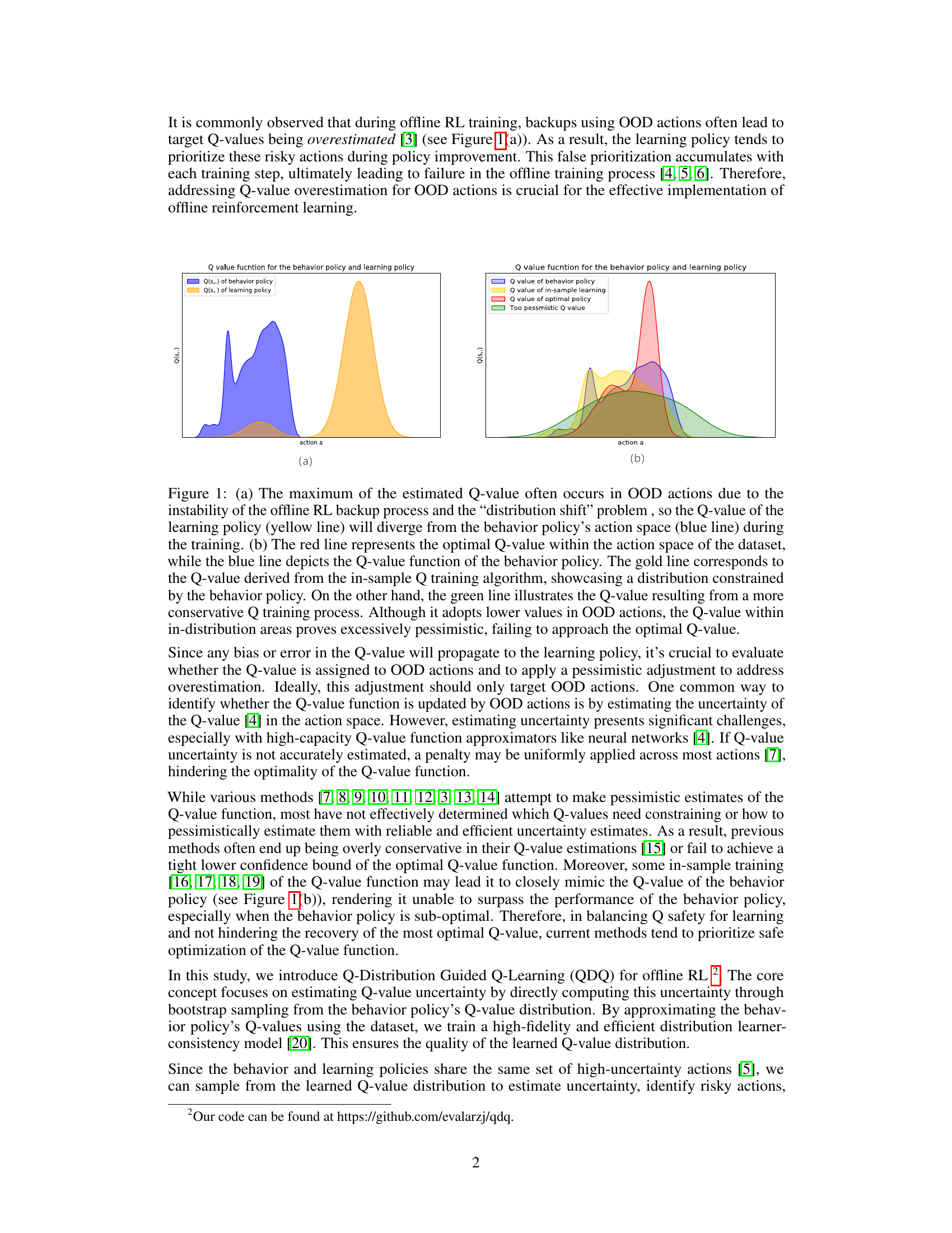
🔼 This figure illustrates the challenges in offline reinforcement learning caused by distribution shift. Panel (a) shows how Q-value overestimation in out-of-distribution (OOD) actions leads to a learning policy diverging from the behavior policy. Panel (b) highlights the trade-off between pessimism (avoiding overestimation) and optimism (approaching the optimal policy), showing that overly conservative methods may hinder performance.
read the caption
Figure 1: (a) The maximum of the estimated Q-value often occurs in OOD actions due to the instability of the offline RL backup process and the “distribution shift” problem, so the Q-value of the learning policy (yellow line) will diverge from the behavior policy's action space (blue line) during the training. (b) The red line represents the optimal Q-value within the action space of the dataset, while the blue line depicts the Q-value function of the behavior policy. The gold line corresponds to the Q-value derived from the in-sample Q training algorithm, showcasing a distribution constrained by the behavior policy. On the other hand, the green line illustrates the Q-value resulting from a more conservative Q training process. Although it adopts lower values in OOD actions, the Q-value within in-distribution areas proves excessively pessimistic, failing to approach the optimal Q-value.

🔼 This table compares the performance of the proposed QDQ algorithm with several state-of-the-art offline reinforcement learning algorithms on three MuJoCo tasks from the D4RL benchmark. The results are presented for different dataset variations (medium, replay, expert) and averaged over five random seeds. The table highlights QDQ’s performance relative to other methods.
read the caption
Table 1: Comparison of QDQ and the other baselines on the three Gym-MuJoCo tasks. All the experiment are performed on the MuJoCo '-v2' dataset. The results are calculated over 5 random seeds.med = medium, r = replay, e = expert, ha = halfcheetah, wa = walker2d, ho=hopper
In-depth insights#
Offline RL’s Q-Issue#
Offline reinforcement learning (RL) faces a critical challenge known as the “Q-issue,” stemming from the inherent limitations of learning solely from offline datasets. Distribution shift, where the data distribution of the behavior policy differs from that of the target learning policy, is a major culprit. This leads to overestimation of Q-values for out-of-distribution (OOD) actions, causing the agent to favor risky actions that are not supported by the offline data. Pessimistic Q-learning methods try to mitigate this by underestimating Q-values, but often become overly conservative, hindering performance. Uncertainty estimation plays a crucial role in addressing the Q-issue; accurately identifying and penalizing high-uncertainty Q-values is vital for safe and effective learning. However, reliable uncertainty estimation remains a significant hurdle. Therefore, robust solutions must balance the need for safe Q-value estimation with the ability to still learn effectively from the available data, successfully navigating this core challenge in offline RL.
QDQ’s Uncertainty#
The core of QDQ’s approach lies in its innovative handling of uncertainty, particularly in the context of offline reinforcement learning. It directly estimates uncertainty by sampling from a learned Q-value distribution, a significant departure from traditional methods. This distribution is learned via a high-fidelity consistency model, which offers several advantages: efficiency and robustness in high-dimensional spaces. The estimation of uncertainty is not only efficient but also effective in identifying risky actions—those prone to overestimation—enabling QDQ to apply a carefully calibrated pessimistic penalty to those actions. This is a clever strategy because it addresses overestimation without introducing excessive conservatism, which is a common pitfall of alternative methods. By combining this sophisticated uncertainty measurement with an uncertainty-aware optimization objective, QDQ achieves a robust balance between optimism and pessimism, allowing it to effectively learn a high-performing policy even from limited, potentially biased offline data. The theoretical analysis further supports the soundness of the approach, adding to its credibility.
Consistency Models#
Consistency models, in the context of offline reinforcement learning, represent a significant advancement in addressing the challenge of uncertainty estimation for Q-values. Unlike traditional methods which may struggle with accuracy and efficiency, especially in high-dimensional spaces, consistency models offer a high-fidelity approach. Their self-consistency property ensures that each step in a sample generation trajectory aligns with the target sample, leading to more reliable uncertainty estimates. This is particularly crucial in offline RL where accurate uncertainty quantification is key to preventing overestimation of Q-values for out-of-distribution actions, a phenomenon that often leads to poor performance. The one-step sampling process of consistency models further enhances computational efficiency, unlike the multi-step processes found in diffusion models. The use of consistency models enables more accurate risk assessment of actions, allowing for more informed and effective pessimistic adjustments to Q-values, ultimately leading to improved policy learning and better performance in offline RL tasks.
Q-Distribution Learn#
A hypothetical ‘Q-Distribution Learn’ section in a reinforcement learning paper would likely detail methods for learning the distribution of Q-values, rather than just their expected values. This is crucial for offline RL because uncertainty estimation is essential for identifying and mitigating the risks of out-of-distribution (OOD) actions, which lead to overestimation of Q-values and suboptimal policies. The section would likely discuss techniques like bootstrapping, creating multiple Q-value estimators to capture variability, or using distributional RL methods that explicitly model the entire Q-value distribution. A key challenge is efficiently and accurately representing the distribution, especially in high-dimensional state-action spaces. Consistency models may be proposed as an efficient approach. The section would highlight theoretical guarantees of the chosen approach, focusing on the accuracy of distribution estimation and how that translates to improved policy learning performance. Finally, experimental results demonstrating the effectiveness of the proposed Q-distribution learning method compared to other uncertainty estimation techniques would be presented.
Future of QDQ#
The future of Q-Distribution Guided Q-Learning (QDQ) appears bright, given its strong performance on benchmark offline reinforcement learning tasks. Further research should focus on improving the consistency model, perhaps through incorporating more sophisticated architectures or training techniques to enhance its accuracy and efficiency, particularly in high-dimensional state spaces. Addressing the sensitivity of QDQ to hyperparameter tuning is also crucial. While the paper demonstrates some robustness, a more automated or adaptive approach to hyperparameter selection would significantly improve usability. Finally, extending QDQ to handle more complex settings, such as continuous action spaces with stochasticity or partially observable environments, would broaden its applicability. Investigating the theoretical guarantees of QDQ in these settings and further empirical validations on diverse tasks remain key future directions. Exploring the integration of QDQ with other advanced offline RL techniques, such as model-based methods or techniques for addressing distribution shift beyond uncertainty penalization, is another promising avenue for advancing the state-of-the-art in offline RL.
More visual insights#
More on figures
🔼 This figure illustrates the problem of Q-value overestimation in offline RL. Panel (a) shows how the learning policy’s Q-value diverges from the behavior policy’s in out-of-distribution (OOD) regions due to overestimation. Panel (b) compares different Q-value learning approaches, highlighting the trade-off between pessimism (avoiding OOD overestimation) and accuracy (approaching the optimal Q-value).
read the caption
Figure 1: (a) The maximum of the estimated Q-value often occurs in OOD actions due to the instability of the offline RL backup process and the “distribution shift” problem, so the Q-value of the learning policy (yellow line) will diverge from the behavior policy's action space (blue line) during the training. (b) The red line represents the optimal Q-value within the action space of the dataset, while the blue line depicts the Q-value function of the behavior policy. The gold line corresponds to the Q-value derived from the in-sample Q training algorithm, showcasing a distribution constrained by the behavior policy. On the other hand, the green line illustrates the Q-value resulting from a more conservative Q training process. Although it adopts lower values in OOD actions, the Q-value within in-distribution areas proves excessively pessimistic, failing to approach the optimal Q-value.

🔼 This figure illustrates two key problems in offline RL. (a) shows how Q-value overestimation in out-of-distribution (OOD) actions leads to divergence between the learning policy and the behavior policy. (b) demonstrates the trade-off between being overly pessimistic in OOD regions and underestimating Q-values in the in-distribution region.
read the caption
Figure 1: (a) The maximum of the estimated Q-value often occurs in OOD actions due to the instability of the offline RL backup process and the “distribution shift” problem, so the Q-value of the learning policy (yellow line) will diverge from the behavior policy's action space (blue line) during the training. (b) The red line represents the optimal Q-value within the action space of the dataset, while the blue line depicts the Q-value function of the behavior policy. The gold line corresponds to the Q-value derived from the in-sample Q training algorithm, showcasing a distribution constrained by the behavior policy. On the other hand, the green line illustrates the Q-value resulting from a more conservative Q training process. Although it adopts lower values in OOD actions, the Q-value within in-distribution areas proves excessively pessimistic, failing to approach the optimal Q-value.

🔼 This figure illustrates the problem of Q-value overestimation in offline reinforcement learning. Panel (a) shows how the learning policy’s Q-values diverge from the behavior policy’s action space in out-of-distribution (OOD) regions, leading to the prioritization of risky actions. Panel (b) compares different Q-value training approaches, highlighting the challenges of balancing safety (pessimistic estimates in OOD regions) with optimality (approaching the optimal Q-value in the in-distribution region).
read the caption
Figure 1: (a) The maximum of the estimated Q-value often occurs in OOD actions due to the instability of the offline RL backup process and the “distribution shift” problem, so the Q-value of the learning policy (yellow line) will diverge from the behavior policy’s action space (blue line) during the training. (b) The red line represents the optimal Q-value within the action space of the dataset, while the blue line depicts the Q-value function of the behavior policy. The gold line corresponds to the Q-value derived from the in-sample Q training algorithm, showcasing a distribution constrained by the behavior policy. On the other hand, the green line illustrates the Q-value resulting from a more conservative Q training process. Although it adopts lower values in OOD actions, the Q-value within in-distribution areas proves excessively pessimistic, failing to approach the optimal Q-value.
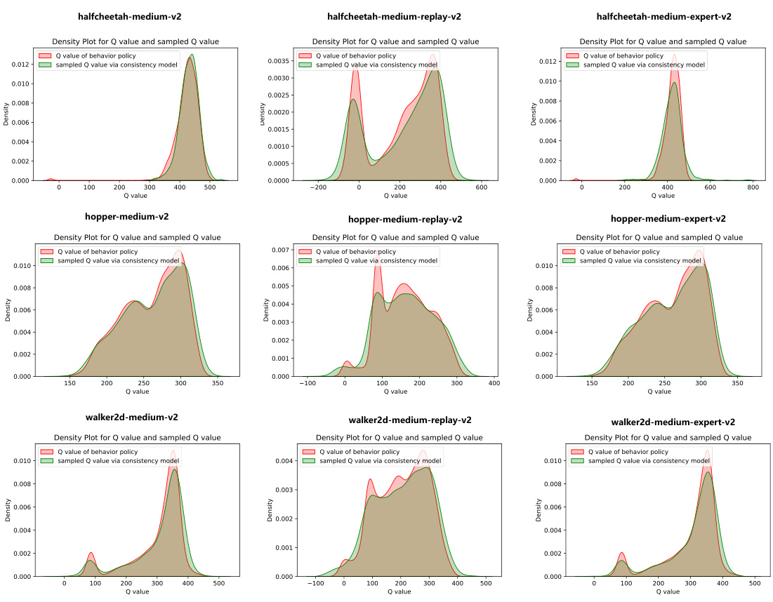
🔼 This figure shows two plots illustrating the challenges of offline reinforcement learning. The left plot (a) demonstrates how Q-value overestimation in out-of-distribution (OOD) regions can lead to the learning policy prioritizing risky actions. The right plot (b) compares the Q-values of an optimal policy, the behavior policy, and learning policies using different training approaches. It highlights the difficulty of balancing safety (pessimism in OOD regions) and accuracy (approaching optimal Q-values in the data distribution).
read the caption
Figure 1: (a) The maximum of the estimated Q-value often occurs in OOD actions due to the instability of the offline RL backup process and the “distribution shift” problem, so the Q-value of the learning policy (yellow line) will diverge from the behavior policy's action space (blue line) during the training. (b) The red line represents the optimal Q-value within the action space of the dataset, while the blue line depicts the Q-value function of the behavior policy. The gold line corresponds to the Q-value derived from the in-sample Q training algorithm, showcasing a distribution constrained by the behavior policy. On the other hand, the green line illustrates the Q-value resulting from a more conservative Q training process. Although it adopts lower values in OOD actions, the Q-value within in-distribution areas proves excessively pessimistic, failing to approach the optimal Q-value.
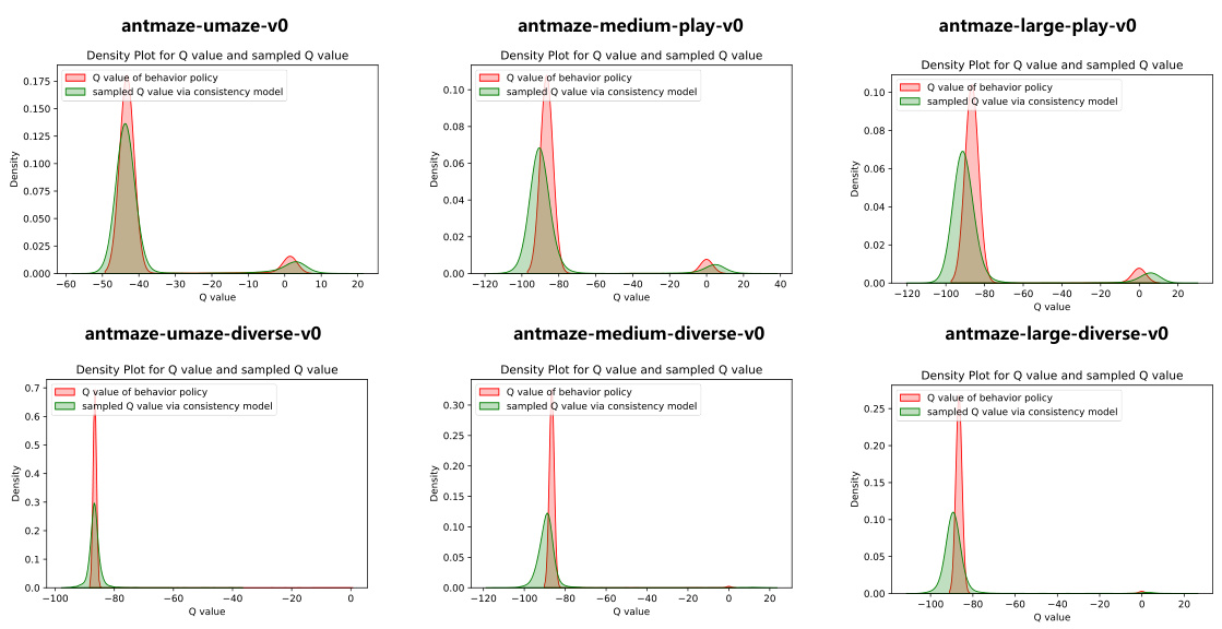
🔼 This figure illustrates the challenges in offline reinforcement learning due to the distribution shift problem. (a) shows how Q-value overestimation in out-of-distribution (OOD) actions can lead the learning policy astray. (b) contrasts the optimal Q-value with the behavior policy’s Q-value and demonstrates the trade-off between pessimism and accuracy in addressing the OOD issue.
read the caption
Figure 1: (a) The maximum of the estimated Q-value often occurs in OOD actions due to the instability of the offline RL backup process and the “distribution shift” problem, so the Q-value of the learning policy (yellow line) will diverge from the behavior policy's action space (blue line) during the training. (b) The red line represents the optimal Q-value within the action space of the dataset, while the blue line depicts the Q-value function of the behavior policy. The gold line corresponds to the Q-value derived from the in-sample Q training algorithm, showcasing a distribution constrained by the behavior policy. On the other hand, the green line illustrates the Q-value resulting from a more conservative Q training process. Although it adopts lower values in OOD actions, the Q-value within in-distribution areas proves excessively pessimistic, failing to approach the optimal Q-value.
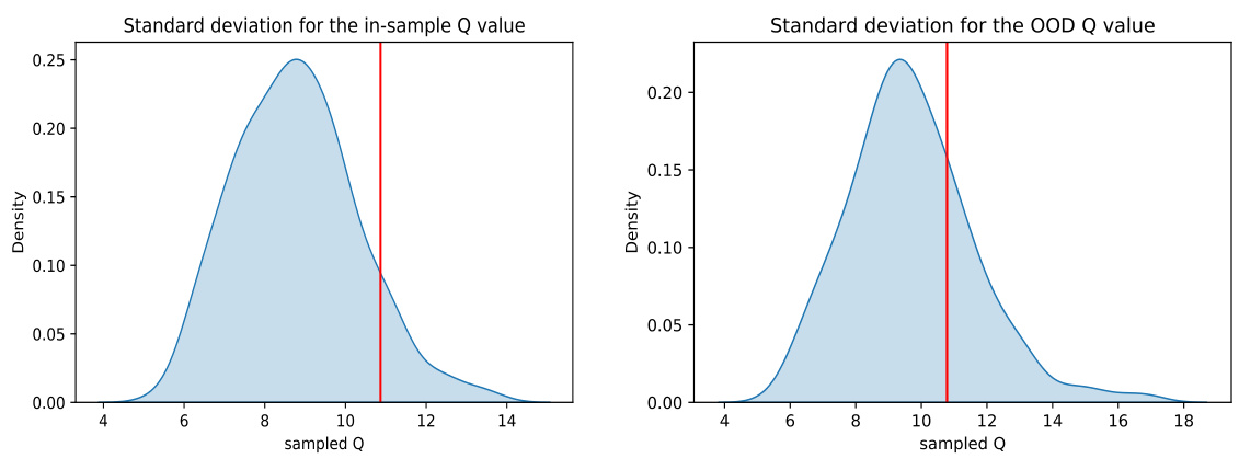
🔼 This figure illustrates the challenges of offline RL training due to distribution shift. Panel (a) shows how Q-value overestimation in out-of-distribution (OOD) actions leads to the learning policy prioritizing risky actions, ultimately hindering performance. Panel (b) highlights the difficulty of balancing Q-value safety and optimality: overly pessimistic adjustments can hinder performance while overly optimistic ones lead to overestimation issues.
read the caption
Figure 1: (a) The maximum of the estimated Q-value often occurs in OOD actions due to the instability of the offline RL backup process and the “distribution shift” problem, so the Q-value of the learning policy (yellow line) will diverge from the behavior policy's action space (blue line) during the training. (b) The red line represents the optimal Q-value within the action space of the dataset, while the blue line depicts the Q-value function of the behavior policy. The gold line corresponds to the Q-value derived from the in-sample Q training algorithm, showcasing a distribution constrained by the behavior policy. On the other hand, the green line illustrates the Q-value resulting from a more conservative Q training process. Although it adopts lower values in OOD actions, the Q-value within in-distribution areas proves excessively pessimistic, failing to approach the optimal Q-value.
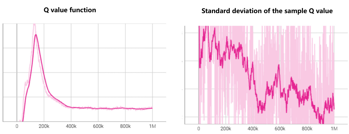
🔼 This figure shows two plots illustrating the problem of Q-value overestimation in offline reinforcement learning. (a) shows how the maximum Q-value often occurs for out-of-distribution (OOD) actions due to the distribution shift problem. (b) compares different Q-value functions, including the optimal Q-value, behavior policy’s Q-value, in-sample Q-learning Q-value, and a more conservative Q-learning Q-value, highlighting the challenges of balancing safety and optimality.
read the caption
Figure 1: (a) The maximum of the estimated Q-value often occurs in OOD actions due to the instability of the offline RL backup process and the “distribution shift” problem, so the Q-value of the learning policy (yellow line) will diverge from the behavior policy's action space (blue line) during the training. (b) The red line represents the optimal Q-value within the action space of the dataset, while the blue line depicts the Q-value function of the behavior policy. The gold line corresponds to the Q-value derived from the in-sample Q training algorithm, showcasing a distribution constrained by the behavior policy. On the other hand, the green line illustrates the Q-value resulting from a more conservative Q training process. Although it adopts lower values in OOD actions, the Q-value within in-distribution areas proves excessively pessimistic, failing to approach the optimal Q-value.
🔼 This figure illustrates two common problems in offline reinforcement learning. (a) shows how Q-value overestimation in out-of-distribution (OOD) actions can cause the learning policy to diverge from the behavior policy. (b) shows that overly conservative Q-value estimations, while avoiding overestimation, can be overly pessimistic and fail to reach optimal Q-values.
read the caption
Figure 1: (a) The maximum of the estimated Q-value often occurs in OOD actions due to the instability of the offline RL backup process and the “distribution shift” problem, so the Q-value of the learning policy (yellow line) will diverge from the behavior policy's action space (blue line) during the training. (b) The red line represents the optimal Q-value within the action space of the dataset, while the blue line depicts the Q-value function of the behavior policy. The gold line corresponds to the Q-value derived from the in-sample Q training algorithm, showcasing a distribution constrained by the behavior policy. On the other hand, the green line illustrates the Q-value resulting from a more conservative Q training process. Although it adopts lower values in OOD actions, the Q-value within in-distribution areas proves excessively pessimistic, failing to approach the optimal Q-value.
🔼 This figure illustrates two key issues in offline reinforcement learning. Subfigure (a) shows how Q-value overestimation in out-of-distribution (OOD) actions leads to the learning policy prioritizing risky actions, causing divergence from the behavior policy’s action space. Subfigure (b) compares the optimal Q-value, behavior policy Q-value, in-sample trained Q-value and a more conservative Q-value. It demonstrates the challenge of balancing safety (pessimism in OOD regions) and optimality (approaching optimal Q-values in the data distribution).
read the caption
Figure 1: (a) The maximum of the estimated Q-value often occurs in OOD actions due to the instability of the offline RL backup process and the “distribution shift” problem, so the Q-value of the learning policy (yellow line) will diverge from the behavior policy's action space (blue line) during the training. (b) The red line represents the optimal Q-value within the action space of the dataset, while the blue line depicts the Q-value function of the behavior policy. The gold line corresponds to the Q-value derived from the in-sample Q training algorithm, showcasing a distribution constrained by the behavior policy. On the other hand, the green line illustrates the Q-value resulting from a more conservative Q training process. Although it adopts lower values in OOD actions, the Q-value within in-distribution areas proves excessively pessimistic, failing to approach the optimal Q-value.
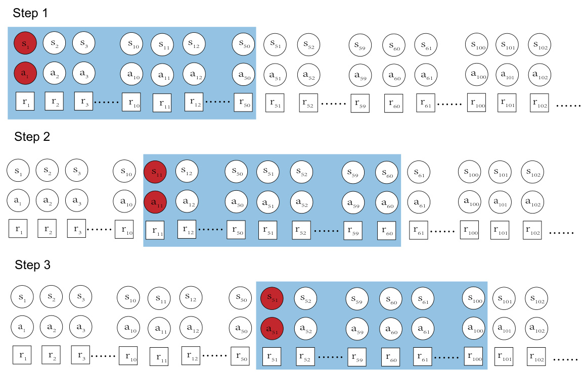
🔼 This figure shows the effect of different sliding window step sizes (k=1, k=10, k=50) on the distribution of the derived Q-values. A smaller step size leads to a more concentrated Q-value distribution, while a larger step size results in a sparser distribution. The window width (T) is held constant at 200 across all three scenarios. The Q-values are normalized for easier comparison.
read the caption
Figure G.1: The derived Q-value distribution when using difference sliding step and same window width to scan over the trajectory's on halfcheetah-medium dataset.The width of the sliding window is set to 200. The Q-value is scaled to facilitate comparison.

🔼 This figure illustrates the problem of Q-value overestimation in offline reinforcement learning. Panel (a) shows how the learning policy’s Q-values diverge from the behavior policy’s action space in out-of-distribution (OOD) regions, leading to overestimation. Panel (b) compares different Q-value estimation methods, highlighting the challenge of balancing safety (pessimistic estimates) with optimality (approaching the true optimal Q-values).
read the caption
Figure 1: (a) The maximum of the estimated Q-value often occurs in OOD actions due to the instability of the offline RL backup process and the “distribution shift” problem, so the Q-value of the learning policy (yellow line) will diverge from the behavior policy's action space (blue line) during the training. (b) The red line represents the optimal Q-value within the action space of the dataset, while the blue line depicts the Q-value function of the behavior policy. The gold line corresponds to the Q-value derived from the in-sample Q training algorithm, showcasing a distribution constrained by the behavior policy. On the other hand, the green line illustrates the Q-value resulting from a more conservative Q training process. Although it adopts lower values in OOD actions, the Q-value within in-distribution areas proves excessively pessimistic, failing to approach the optimal Q-value.

🔼 This figure illustrates the problem of Q-value overestimation in offline RL. (a) shows how the learning policy’s Q-values diverge from the behavior policy’s action space due to overestimation of out-of-distribution (OOD) actions. (b) compares different Q-value training approaches, highlighting the trade-off between pessimism and optimality.
read the caption
Figure 1: (a) The maximum of the estimated Q-value often occurs in OOD actions due to the instability of the offline RL backup process and the “distribution shift” problem, so the Q-value of the learning policy (yellow line) will diverge from the behavior policy's action space (blue line) during the training. (b) The red line represents the optimal Q-value within the action space of the dataset, while the blue line depicts the Q-value function of the behavior policy. The gold line corresponds to the Q-value derived from the in-sample Q training algorithm, showcasing a distribution constrained by the behavior policy. On the other hand, the green line illustrates the Q-value resulting from a more conservative Q training process. Although it adopts lower values in OOD actions, the Q-value within in-distribution areas proves excessively pessimistic, failing to approach the optimal Q-value.
🔼 This figure illustrates the problem of Q-value overestimation in offline reinforcement learning. (a) Shows how the learning policy’s Q-values diverge from the behavior policy’s action space in out-of-distribution (OOD) regions, leading to the selection of risky actions. (b) Compares different Q-value training approaches, highlighting the trade-off between pessimism (avoiding OOD actions) and optimism (approaching optimal performance).
read the caption
Figure 1: (a) The maximum of the estimated Q-value often occurs in OOD actions due to the instability of the offline RL backup process and the “distribution shift” problem, so the Q-value of the learning policy (yellow line) will diverge from the behavior policy's action space (blue line) during the training. (b) The red line represents the optimal Q-value within the action space of the dataset, while the blue line depicts the Q-value function of the behavior policy. The gold line corresponds to the Q-value derived from the in-sample Q training algorithm, showcasing a distribution constrained by the behavior policy. On the other hand, the green line illustrates the Q-value resulting from a more conservative Q training process. Although it adopts lower values in OOD actions, the Q-value within in-distribution areas proves excessively pessimistic, failing to approach the optimal Q-value.
More on tables

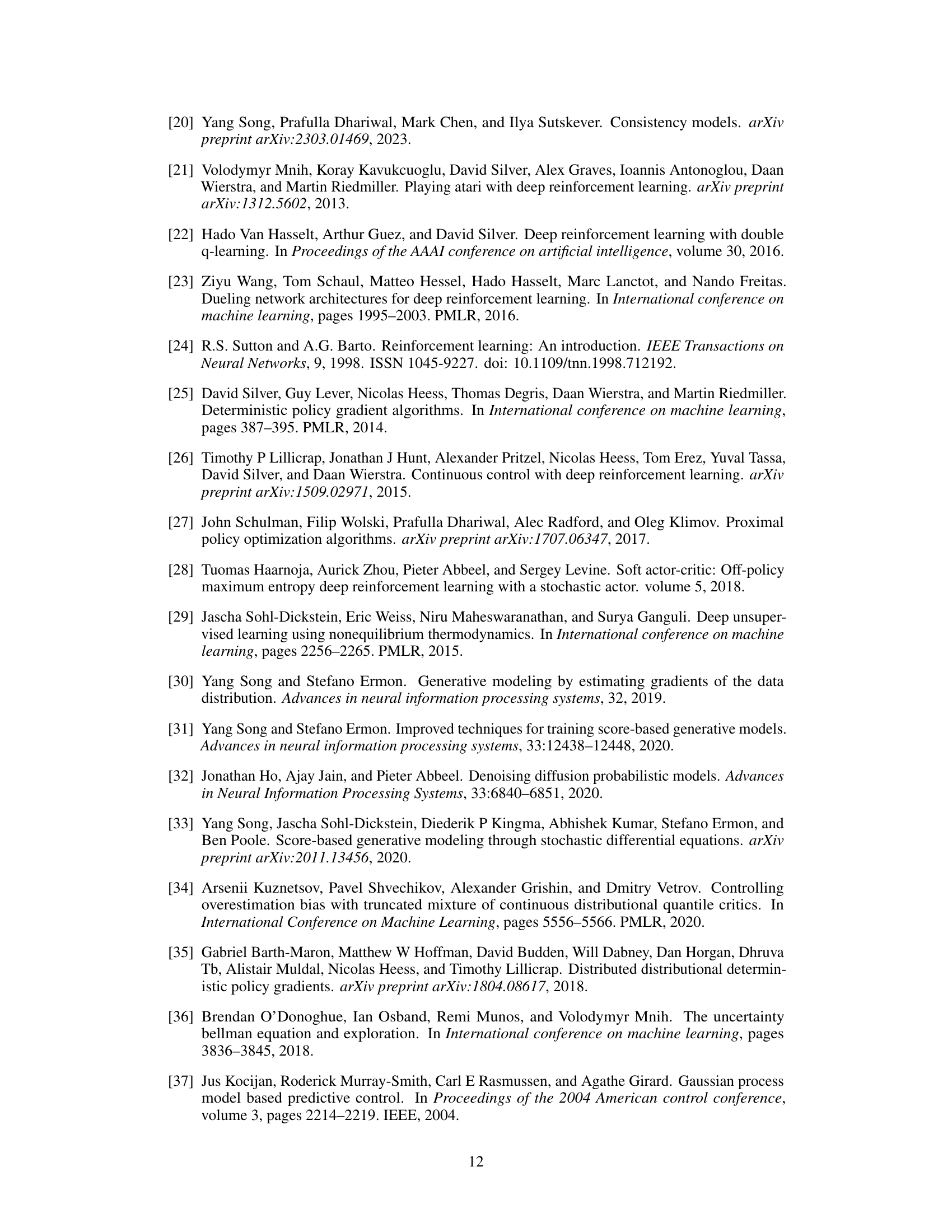
🔼 This table compares the performance of the proposed QDQ algorithm against several other state-of-the-art offline reinforcement learning methods on AntMaze tasks from the D4RL benchmark. The results are shown for different AntMaze environments (umaze, umaze-diverse, medium-play, medium-diverse, large-play, and large-diverse), and the total score is also given. The table indicates the average score over 5 random seeds for each algorithm and environment.
read the caption
Table 2: Comparison of QDQ and the other baselines on the AntMaze tasks. All the experiment are performed on the Antmaze '-v0' dataset for the comparison comfortable with previous baseline. The results are calculated over 5 random seeds.
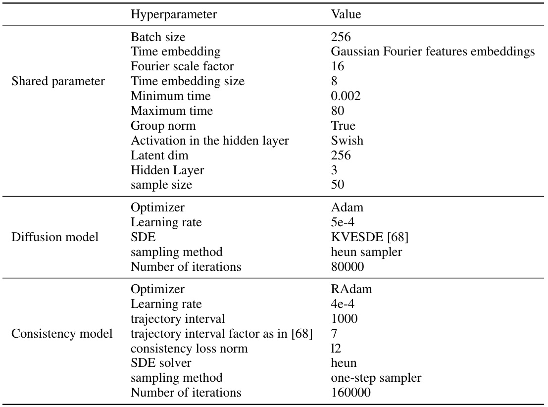
🔼 This table compares the performance of the proposed QDQ algorithm against several state-of-the-art offline reinforcement learning algorithms on three MuJoCo tasks from the D4RL benchmark. The results are averaged across five random seeds and show QDQ’s performance relative to others across different dataset variations (medium, replay, expert). Abbreviations are provided for clarity.
read the caption
Table 1: Comparison of QDQ and the other baselines on the three Gym-MuJoCo tasks. All the experiment are performed on the MuJoCo '-v2' dataset. The results are calculated over 5 random seeds.med = medium, r = replay, e = expert, ha = halfcheetah, wa = walker2d, ho=hopper
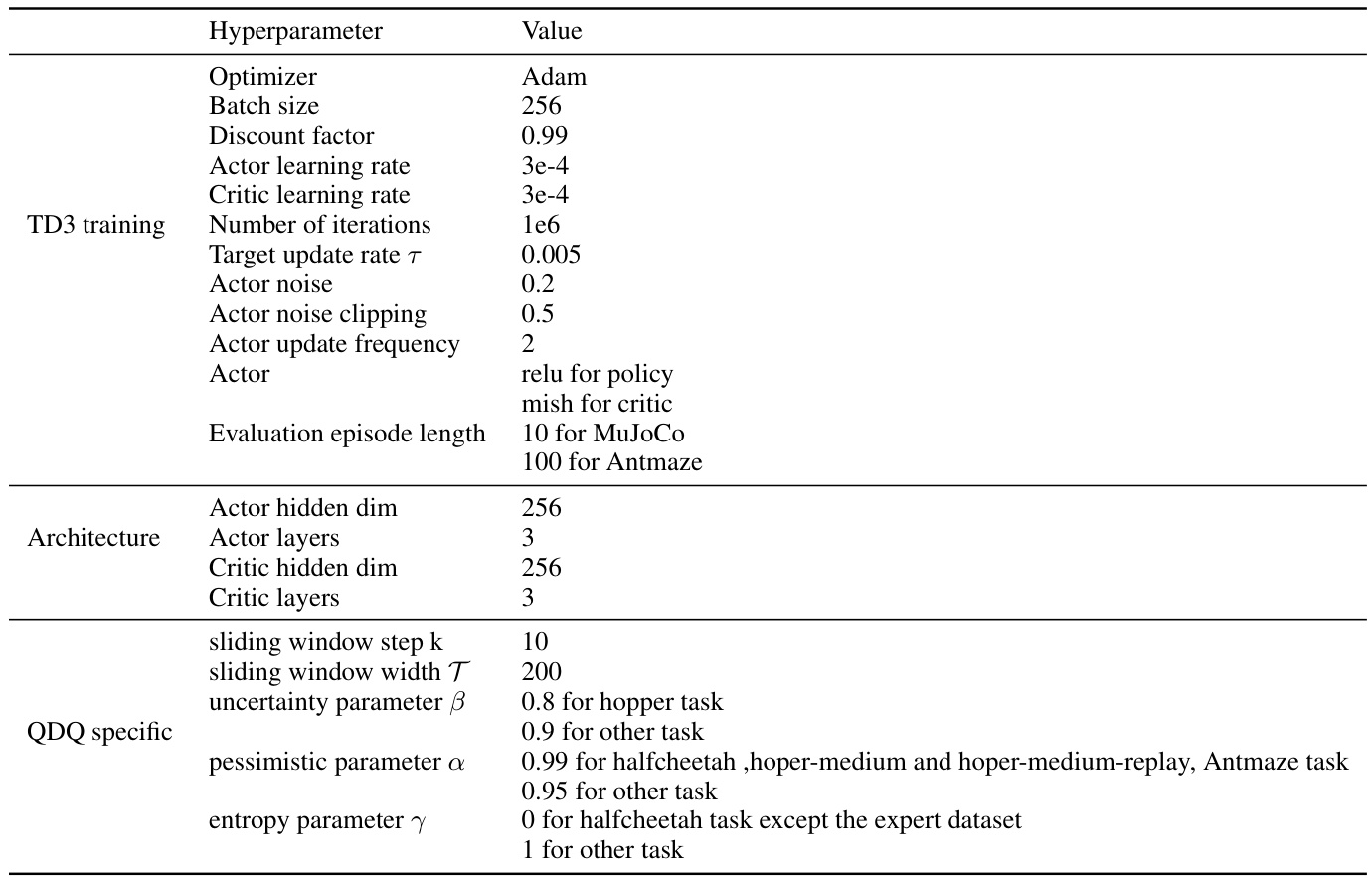
🔼 This table compares the performance of the proposed QDQ algorithm with several state-of-the-art offline reinforcement learning algorithms on three MuJoCo tasks from the D4RL benchmark. The results are presented for different dataset variations (medium, replay, expert) for each task (halfcheetah, hopper, walker2d). The table shows the average normalized scores across 5 random seeds, indicating the relative performance of each algorithm on these tasks and datasets.
read the caption
Table 1: Comparison of QDQ and the other baselines on the three Gym-MuJoCo tasks. All the experiment are performed on the MuJoCo '-v2' dataset. The results are calculated over 5 random seeds.med = medium, r = replay, e = expert, ha = halfcheetah, wa = walker2d, ho=hopper
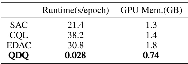
🔼 This table compares the performance of the proposed QDQ algorithm against other state-of-the-art offline reinforcement learning methods on three MuJoCo tasks from the D4RL benchmark. It shows the average normalized scores achieved by each algorithm across five random seeds, with results broken down by dataset type (medium, replay, expert) for each task.
read the caption
Table 1: Comparison of QDQ and the other baselines on the three Gym-MuJoCo tasks. All the experiment are performed on the MuJoCo '-v2' dataset. The results are calculated over 5 random seeds.med = medium, r = replay, e = expert, ha = halfcheetah, wa = walker2d, ho=hopper
Full paper#
