↗ OpenReview ↗ NeurIPS Homepage ↗ Chat
TL;DR#
Training large deep neural networks is computationally expensive, particularly when using second-order optimization methods like natural gradient descent which offer superior convergence properties. These methods often involve calculating and inverting the Fisher information matrix, a process that scales poorly with model size. Approximations exist but often sacrifice accuracy.
This paper introduces a new optimizer called Layer-wise Natural Gradient Descent (LNGD) to tackle this issue. LNGD cleverly approximates the Fisher information matrix in a layer-wise fashion, reducing computation while preserving key information. This is further enhanced by a novel adaptive layer-wise learning rate which further accelerates training. The authors provide a global convergence analysis to support their claims. Extensive experiments confirm that LNGD is competitive with state-of-the-art methods, achieving faster convergence and higher accuracy on several image classification and machine translation tasks.
Key Takeaways#
Why does it matter?#
This paper is important because it offers a novel solution to a critical challenge in deep learning: the high computational cost of second-order optimization methods. By introducing LNGD, it provides a computationally efficient alternative to existing methods, accelerating the training process and improving model performance. This is particularly relevant in the context of increasingly large and complex deep learning models, where training time is a major bottleneck. The adaptive layer-wise learning rate mechanism and convergence analysis also offer valuable insights for researchers working on optimizer development and optimization theory. This opens new avenues for research in efficient optimization strategies and further improvements in the training of deep neural networks.
Visual Insights#

This figure compares the exact Fisher information matrix (F) with the approximation (FLNGD) proposed by the authors. The top row shows the entire 400x400 matrix for the first layer of a neural network trained on MNIST. The bottom row shows a zoomed-in 40x40 section of the top matrices. The left column shows the exact matrix F, the middle column displays the approximation FLNGD, and the right column shows the absolute error between them, with brighter colors indicating larger errors.

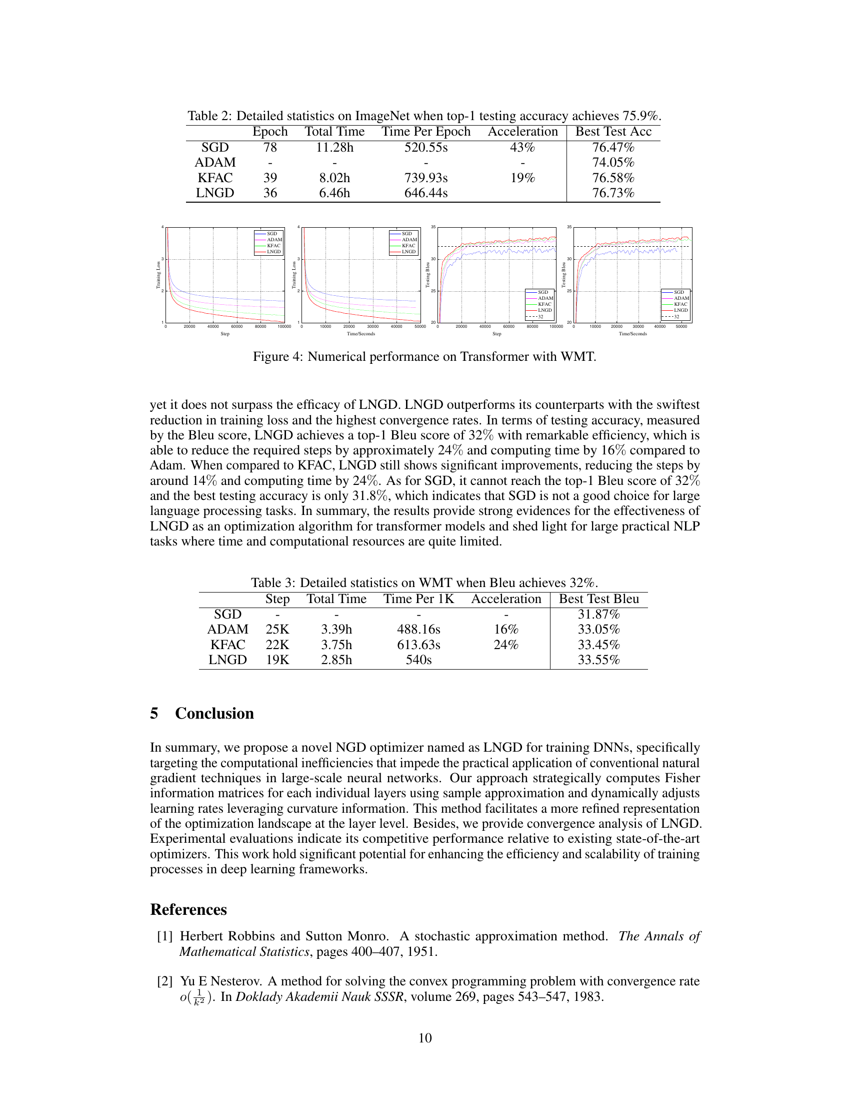
This table presents a quantitative comparison of different optimization algorithms on the ImageNet dataset. The metrics reported include the number of epochs required to reach a top-1 testing accuracy of 75.9%, the total training time, the time per epoch, the acceleration achieved relative to SGD (Stochastic Gradient Descent), and the best test accuracy reached.
In-depth insights#
LNGD Optimizer#
The LNGD optimizer, a novel layer-wise natural gradient descent method, presents a compelling approach to training deep neural networks. Its core innovation lies in a two-step approximation of the Fisher information matrix, drastically reducing computational costs associated with traditional second-order optimization methods. Firstly, a layer-wise sampling technique efficiently computes block diagonal components, bypassing complete backpropagation. Secondly, a Kronecker product approximation, preserving trace equality, further simplifies calculations. The introduction of an adaptive layer-wise learning rate further enhances performance. While the theoretical analysis establishes global convergence under certain assumptions, the empirical results on image classification and machine translation tasks demonstrate strong competitiveness against state-of-the-art methods. LNGD’s efficiency gains stem from its intelligent approximations, making it a practical solution for large-scale deep learning applications, although the assumptions made might limit generalizability.
Layer-wise Sampling#
Layer-wise sampling, as a conceptual approach, presents a compelling strategy to optimize the training of deep neural networks. The core idea involves computing the Fisher information matrix, crucial for natural gradient descent, in a layer-by-layer fashion. This contrasts with traditional methods that compute the matrix globally, leading to significant computational bottlenecks, especially with larger models. By decomposing the computation, layer-wise sampling drastically reduces the computational cost because it only requires partial backpropagation for each layer’s local information, instead of a complete pass through the whole network. Efficiency gains are paramount, as the algorithm avoids unnecessary calculations involving parameters that are not directly relevant to the layer being processed at the moment. While approximations are often necessary in practice to further improve efficiency, the inherent advantage of this approach is the reduction in computation complexity. However, designing effective approximation strategies that accurately represent the relevant information within each layer’s context is critical to the method’s success. Careful consideration must also be given to potential trade-offs between accuracy and efficiency when applying approximation techniques. The impact on convergence speed and overall performance needs to be analyzed thoroughly as this optimization technique changes the learning dynamics compared to traditional global methods. Ultimately, the success of layer-wise sampling hinges on its ability to maintain sufficient accuracy of the Fisher Information Matrix while dramatically reducing computational costs during training.
Adaptive Learning#
Adaptive learning methods, crucial for optimizing deep neural networks, dynamically adjust parameters during training, enhancing efficiency and performance. The core concept lies in tailoring learning rates to individual parameters or groups of parameters, unlike traditional methods using a global learning rate. This adaptability is particularly important in deep networks due to varying gradients across layers and the challenge of finding optimal parameters. Adaptive methods achieve this adjustment through various techniques, often incorporating information about the gradient’s magnitude or its past history. These methods can lead to faster convergence, improved generalization, and reduced sensitivity to hyperparameter tuning. However, adaptive methods are not without limitations. They can be more computationally expensive than traditional methods. Furthermore, choosing the right adaptive learning technique requires careful consideration of the specific network architecture, dataset, and task. Therefore, research on adaptive learning remains a vibrant area focusing on refining existing techniques and exploring innovative approaches that strike a balance between computational efficiency and learning performance.
Convergence Analysis#
The convergence analysis section of a research paper is crucial for establishing the reliability and effectiveness of any proposed algorithm or model. A rigorous convergence analysis provides a theoretical guarantee of the algorithm’s ability to reach a solution, or at least a near-optimal solution, within a certain timeframe. The key aspects to look for in a strong convergence analysis are: clearly stated assumptions, a well-defined measure of convergence (e.g., distance to the optimal solution, error rate), and a formal proof of convergence using established mathematical techniques. The proof should demonstrate the rate of convergence (e.g., linear, sublinear, exponential), which offers insights into the algorithm’s efficiency. Assumptions should be carefully examined; oversimplifying assumptions may limit the analysis’s applicability to real-world scenarios. A discussion of the limitations of the analysis, resulting from the assumptions and mathematical simplifications, is essential for a fair and complete assessment. In many machine learning contexts, global convergence is the ultimate goal, meaning the algorithm can converge to a global minimum or maximum regardless of the starting point. However, proving global convergence is often very challenging, and papers may often focus on proving local convergence instead, which is convergence to a local optimum near the initialization point.
Future Enhancements#
Future enhancements for this layer-wise natural gradient descent (LNGD) optimizer could explore several promising avenues. Improving the layer-wise sample approximation is crucial; refining the Gaussian distribution assumption or exploring alternative distributions tailored to different layers or activation functions would enhance accuracy. Developing more sophisticated adaptive learning rate mechanisms beyond the proposed adaptive layer-wise approach, potentially incorporating second-order information or exploring different optimization strategies for learning rates, warrants investigation. Further reducing computational complexity is another priority. This might involve exploring more efficient Kronecker product approximations or leveraging distributed computing techniques more effectively. Extending LNGD to handle diverse network architectures beyond fully connected and convolutional networks, such as recurrent or transformer models, is important to broaden its applicability. Finally, a comprehensive empirical evaluation across a wider range of datasets and tasks, including more extensive ablation studies, would strengthen the method’s overall robustness and provide more definitive conclusions on its practical advantages.
More visual insights#
More on figures

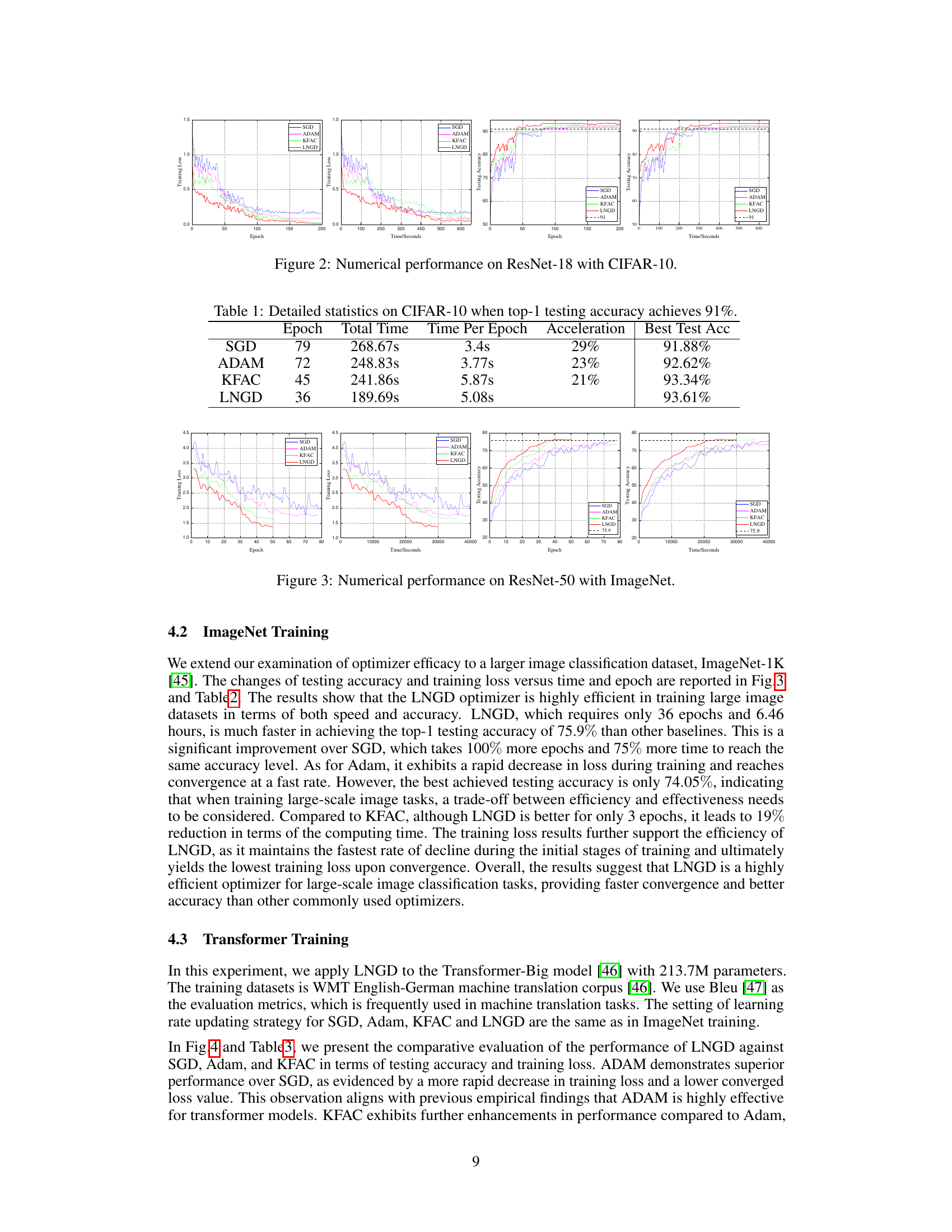
This figure compares the performance of four different optimizers (SGD, Adam, KFAC, and LNGD) on the CIFAR-10 dataset using ResNet-18 architecture. The plots show the training loss and testing accuracy over epochs and training time (in seconds). LNGD demonstrates faster convergence and higher accuracy than the other optimizers.
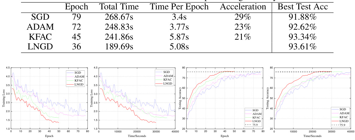
This figure displays the training and testing results of the ResNet-18 model trained on the CIFAR-10 dataset using four different optimizers: SGD, Adam, KFAC, and LNGD. The plots show the changes in training loss and testing accuracy over time (in seconds) and epochs. LNGD demonstrates faster convergence and higher testing accuracy compared to the other optimizers.

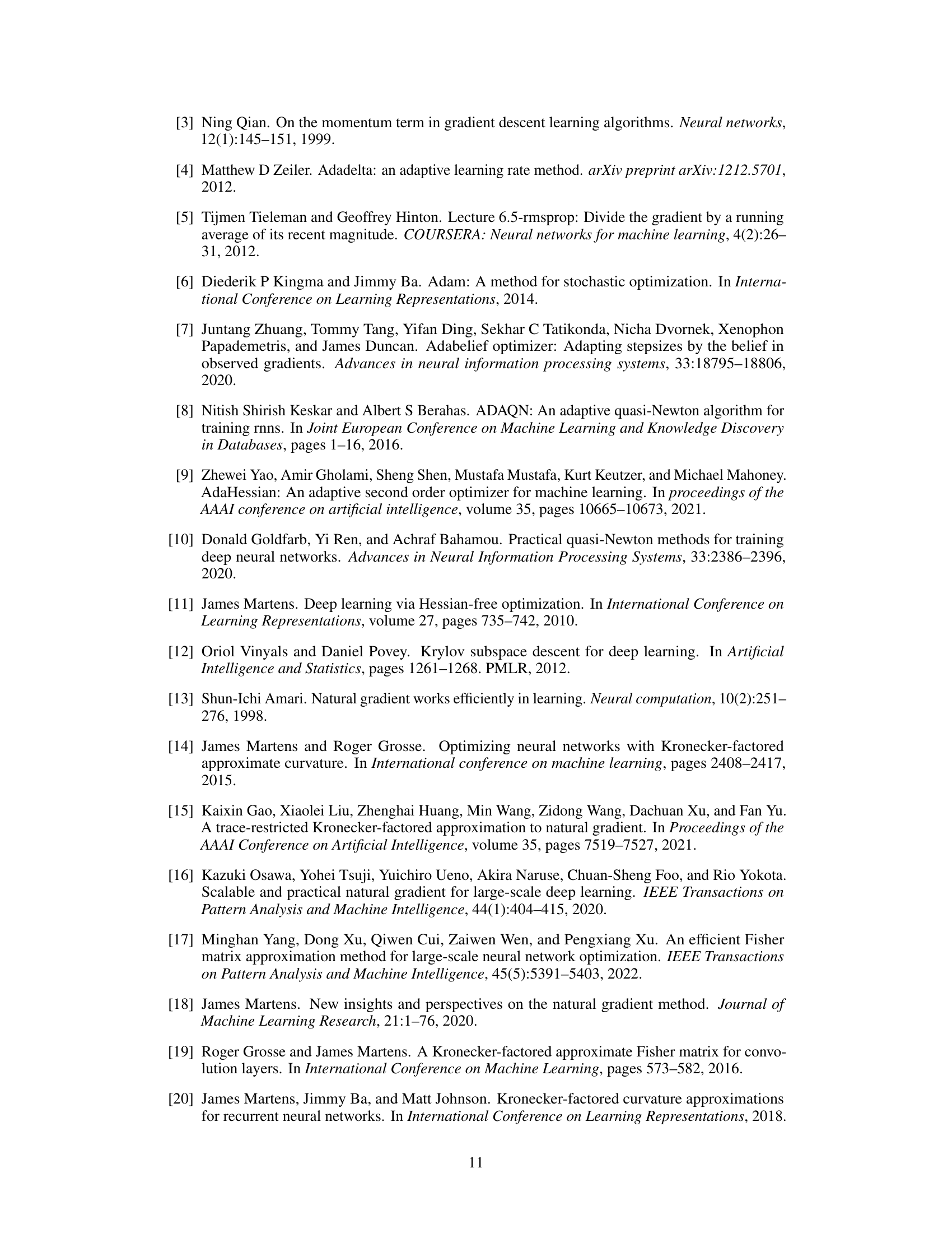
The figure shows the training loss and testing BLEU score (a common metric for machine translation) over training steps and time in seconds for four different optimizers: SGD, Adam, KFAC, and LNGD. The plots illustrate the convergence speed and performance of each optimizer on the WMT English-German machine translation task. LNGD demonstrates faster convergence and better performance compared to the other optimizers.
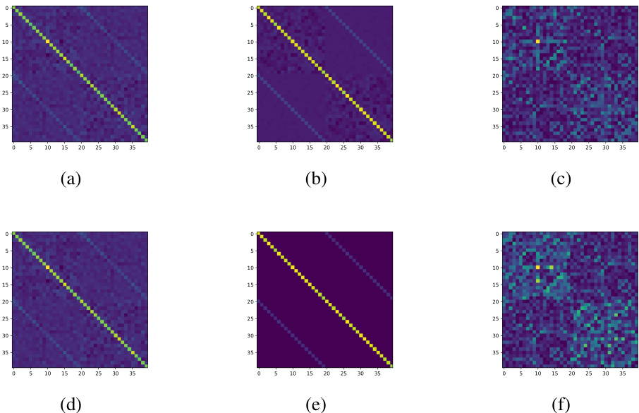
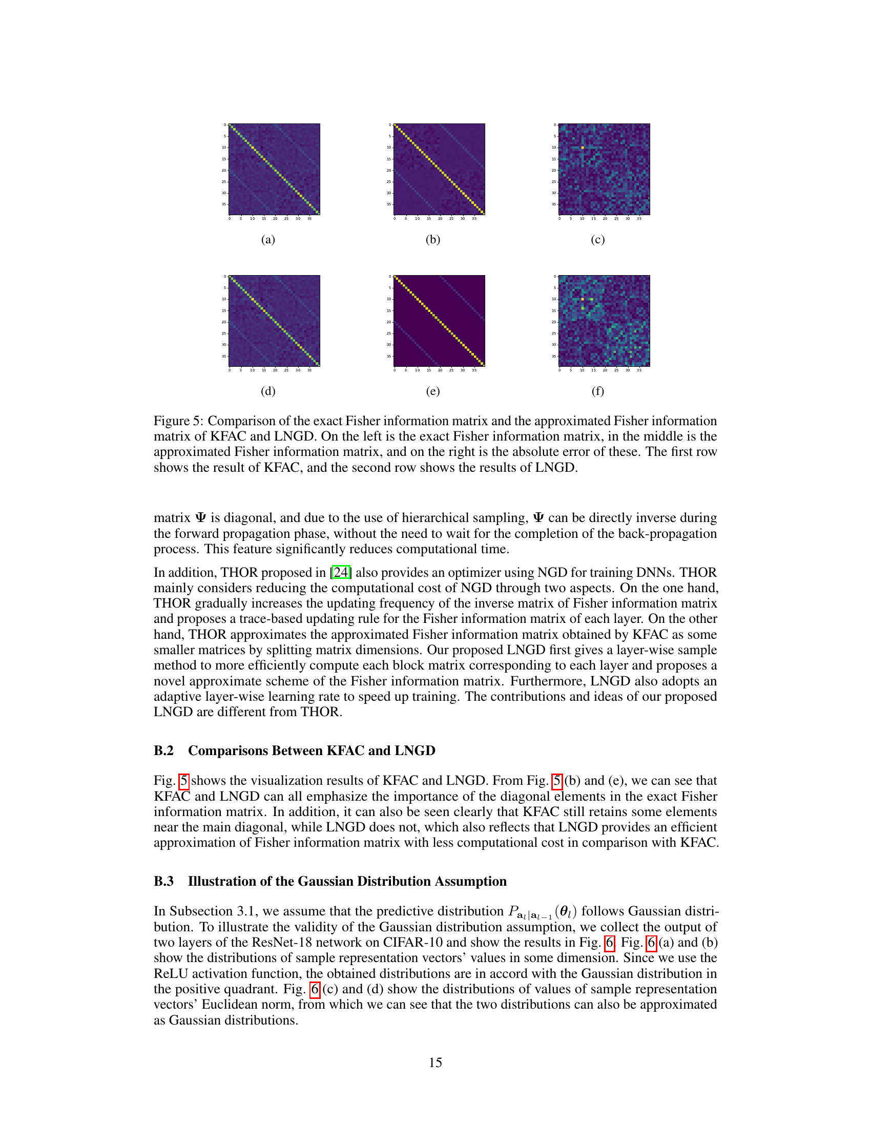
This figure compares the exact Fisher Information Matrix (FIM) with approximations from KFAC and LNGD methods. Each row represents a comparison for a single layer. The left column shows the true FIM; the middle shows the approximation by KFAC (top row) and LNGD (bottom row); and the right shows the absolute difference between the true FIM and the approximation. The visualization helps to understand how well each approximation captures the true FIM, specifically highlighting the diagonal elements as they are particularly emphasized by LNGD.

The figure shows four histograms visualizing the distributions of sample representation vectors’ values in some dimensions and Euclidean norm of two layers of ResNet-18 network on CIFAR-10. The distributions are shown to be approximately Gaussian, supporting the Gaussian distribution assumption used in the layer-wise sample approximation of the Fisher information matrix.
This figure compares the exact Fisher information matrix (F) with the approximation used in the proposed LNGD method (FLNGD). It visualizes the matrices for the first layer of a neural network trained on the MNIST dataset, showcasing both the full 400x400 matrix and a zoomed-in 40x40 section. The rightmost column in each row displays the absolute error between the exact and approximated matrices, highlighting the accuracy of the approximation.
More on tables

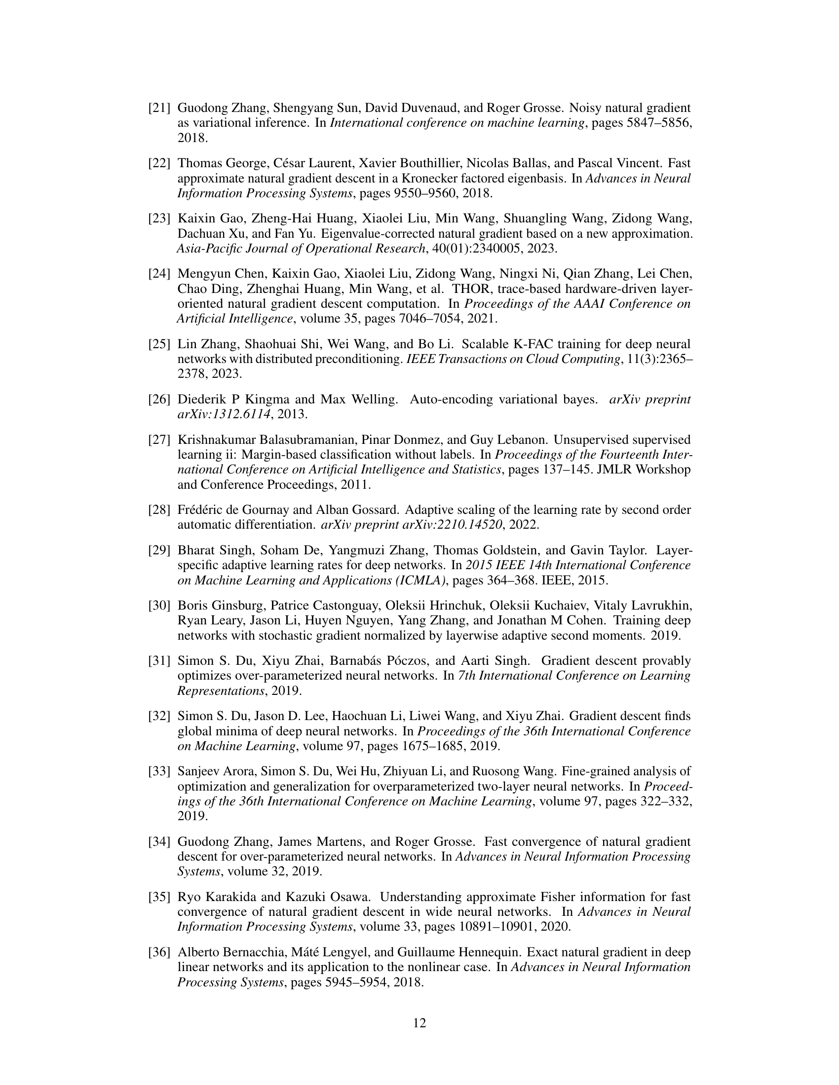
This table shows the detailed statistics of different optimizers on the WMT English-German machine translation corpus when the Bleu score reaches 32%. It compares the number of steps, total time, time per 1K steps, acceleration, and best test Bleu score achieved by SGD, Adam, KFAC, and LNGD. The results highlight LNGD’s efficiency in achieving high Bleu scores with fewer steps and less time compared to other methods.

This table summarizes how different natural gradient descent (NGD) optimizers approximate the Fisher information matrix (F_i) for each layer (i). KFAC uses a Kronecker product of two matrices (A and B). EKFAC refines this by incorporating eigenvalue decomposition and rescaling. TKFAC uses a Kronecker product scaled by a coefficient (δ). LNGD, the proposed method, uses a Kronecker product of matrices (Φ and Ψ), with Ψ being a diagonal matrix.

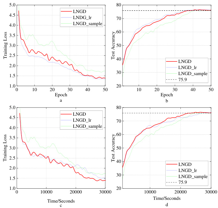
This table presents the results of ablation studies conducted to evaluate the individual contributions of the adaptive layer-wise learning rate and the layer-wise sampling technique within the LNGD optimizer. The results are presented for three versions of the LNGD algorithm: 1. LNGD-lr: Uses the adaptive learning rate but not the layer-wise sampling. 2. LNGD-sample: Uses the layer-wise sampling but not the adaptive learning rate. 3. LNGD: Uses both the adaptive learning rate and the layer-wise sampling. The table shows the number of epochs required to reach a top-1 testing accuracy of 75.9%, the total training time, the training time per epoch, and the relative acceleration compared to the standard LNGD algorithm. It demonstrates the synergistic effect of combining both techniques for faster and more efficient model training.

This table presents a comparison of different optimization methods on the CIFAR-10 dataset for image classification. The comparison focuses on the number of epochs required to reach a top-1 testing accuracy of 91%, the total training time, the time per epoch, and the speedup achieved compared to SGD. The results show that LNGD achieves this accuracy using the fewest epochs and shortest total training time.
Full paper#

