↗ OpenReview ↗ NeurIPS Homepage ↗ Chat
TL;DR#
Traditional methods for studying neural population dynamics often involve passively recording neural activity during a task, leading to inefficient data collection and correlational, rather than causal, inferences. This limits understanding of how neural circuits compute and perform tasks. Moreover, designing effective photostimulation experiments to understand neural circuits is challenging due to the sheer size of the search space and the time-consuming nature of experiments.
This work addresses these challenges by developing active learning techniques that intelligently select which neurons to stimulate, optimizing data collection and causal inference. The researchers use a low-rank linear dynamical systems model to capture the low-dimensional structure of neural population dynamics and propose an active learning procedure to choose informative photostimulation patterns. This method is demonstrated on both real and synthetic data, resulting in substantially more accurate estimates of neural population dynamics with fewer measurements than traditional passive methods.
Key Takeaways#
Why does it matter?#
This paper is crucial for researchers in neuroscience and machine learning because it introduces a novel active learning approach for efficiently identifying neural population dynamics. It bridges the gap between experimental design and theoretical understanding by using two-photon holographic optogenetics, offering a more efficient and targeted way to study brain circuits.
Visual Insights#

This figure demonstrates the experimental setup and data. (a) shows the two-photon imaging and holographic photostimulation platform used to record neural activity and apply targeted photostimulation. (b) shows example time series data: photostimulation inputs (top) and the corresponding neural responses (bottom) from a subset of the recorded neurons. (c) shows the singular value decomposition of the neural activity data, illustrating that the data lies in a low-dimensional subspace.
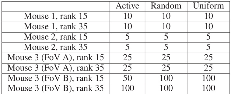
This table shows the nuclear norm constraint values used for each plot in Figure 3. The values were selected to minimize the estimation error for each method (Active, Random, Uniform). The constraints vary across different mouse datasets and ranks of the model, reflecting the different scales and levels of complexity in the data.
In-depth insights#
Active Learning’s Role#
Active learning plays a crucial role in accelerating the identification of neural population dynamics by intelligently selecting informative photostimulation patterns. Instead of passively collecting data, active learning strategically chooses which neurons to stimulate, focusing on those that maximize the information gained about the underlying low-rank structure of the neural dynamics. This targeted approach significantly reduces the amount of experimental data required to reach a given predictive accuracy, making the process more efficient and resource-friendly. The core idea is to leverage low-rank dynamical systems models to identify the most informative stimuli. By actively designing these stimuli, researchers can efficiently learn more accurate models of neural population activity and causal connectivity, thereby providing valuable insights into the computations performed by neural populations and enhancing our understanding of brain circuits.
Low-Rank Dynamics#
The concept of ‘Low-Rank Dynamics’ in neural systems suggests that high-dimensional neural activity can be effectively represented by a lower-dimensional structure. This is particularly valuable for analyzing neural population dynamics, reducing computational complexity and improving the efficiency of model estimation. Low-rank models capture the essential correlations within neural populations, enabling inference of causal interactions despite the high dimensionality of the data. This approach is useful for both simulation and analysis of neural data, leading to more accurate predictions with significantly fewer measurements compared to full-rank methods. Active learning strategies can further refine this by intelligently selecting informative stimuli, accelerating the learning process and maximizing the information obtained from limited experimental resources. This low-rank approach facilitates a deeper understanding of neural computations by focusing on the underlying low-dimensional dynamics that govern neural activity. The ability to capture causal relationships and predict dynamics with limited data is significant for improving our understanding of brain function.
Stimulus Design#
Stimulus design in this research paper focuses on efficiently selecting which neurons to stimulate using two-photon holographic optogenetics. The goal is to maximize the information gained from each experiment, minimizing the amount of data required to accurately model neural population dynamics. This involves developing an active learning procedure that leverages low-rank structure within neural responses to photostimulation. By strategically targeting informative patterns, the researchers aim to significantly reduce the number of trials necessary to build accurate predictive models of the neural population activity, improving overall experimental efficiency and gaining insight into the computations performed by neural populations. The proposed methodology involves using a low-rank autoregressive model to capture low-dimensional structure in the neural data, and then adaptively selecting stimulation patterns that target this structure to maximize information gain. The efficacy of this method is demonstrated on real and synthetic datasets, achieving significant gains compared to passive stimulus selection strategies. A key contribution is the development of a novel active learning procedure for low-rank regression, which has broader implications beyond neuroscience.
Real Data Analysis#
A robust ‘Real Data Analysis’ section would thoroughly evaluate the proposed active learning method’s performance on real-world neural data. It should compare its efficiency against passive baselines, demonstrating improvements in prediction accuracy or data usage. Key metrics should include prediction error, AUROC, and the number of trials needed to reach a specified performance level. The analysis should not just show numerical results, but also provide visualizations such as example predictions and error distributions to showcase model behavior and highlight the practical impact of active learning. Direct comparison to existing state-of-the-art methods is crucial, and the discussion should address whether the improvements are statistically significant. Finally, a discussion of the dataset’s characteristics, potential biases, and limitations is vital for assessing the generalizability of the findings and interpreting the results with appropriate caution. Robustness checks, exploring the sensitivity of results to various parameters and noise levels, will enhance the credibility and impact of the analysis.
Future Directions#
Future research could explore several promising avenues. Extending the active learning framework to nonlinear dynamical systems is crucial, as many real-world neural processes exhibit nonlinearities. Investigating the impact of different noise models and their influence on active learning performance would also be valuable. Developing more sophisticated methods for selecting informative photostimulation patterns that account for both structural and temporal properties of the neural dynamics is a key area for improvement. Finally, bridging the gap between theoretical insights and practical implementation by testing the active learning approach on a wider range of neural systems and experimental paradigms is essential to demonstrate its true potential and assess its generalizability. Furthermore, rigorous analyses of the algorithm’s computational complexity and scalability should be performed to guide future optimizations.
More visual insights#
More on figures
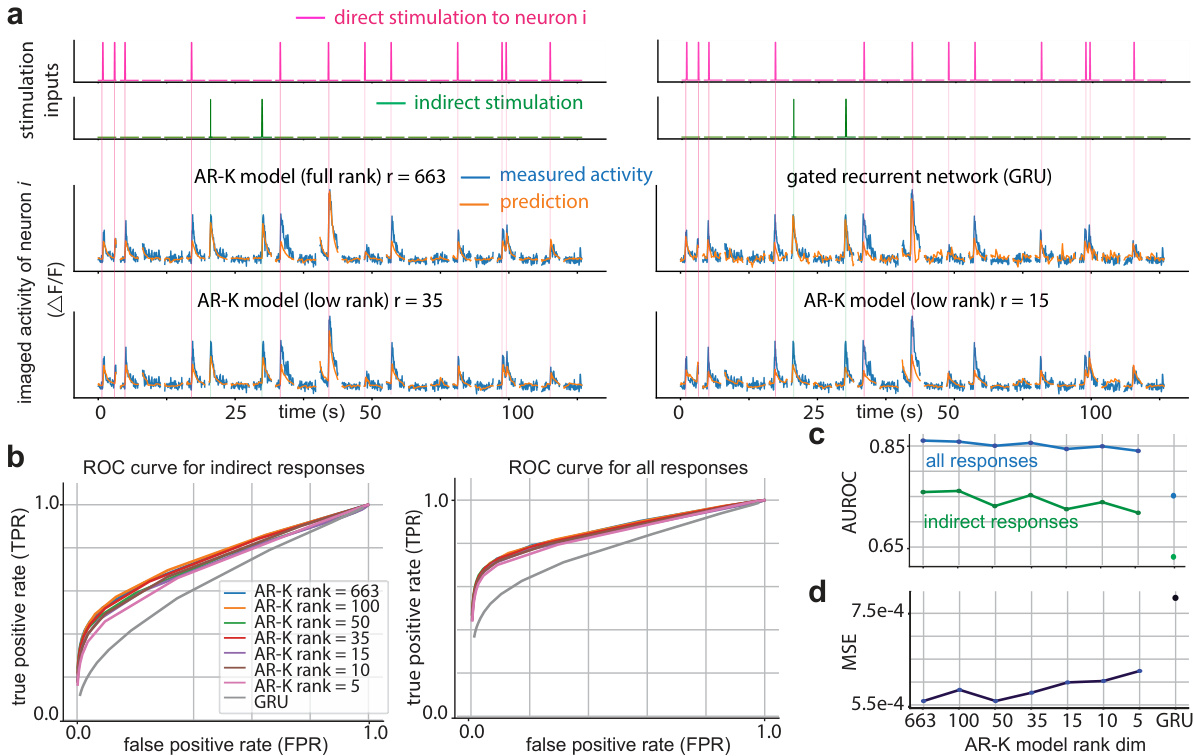
This figure demonstrates the performance of low-rank autoregressive models and GRU networks in predicting neural activity. It shows example predictions compared to actual recordings, ROC curves assessing the models’ ability to identify neural responses (both direct and indirect), and a comparison of AUROC and MSE values across models with varying ranks.
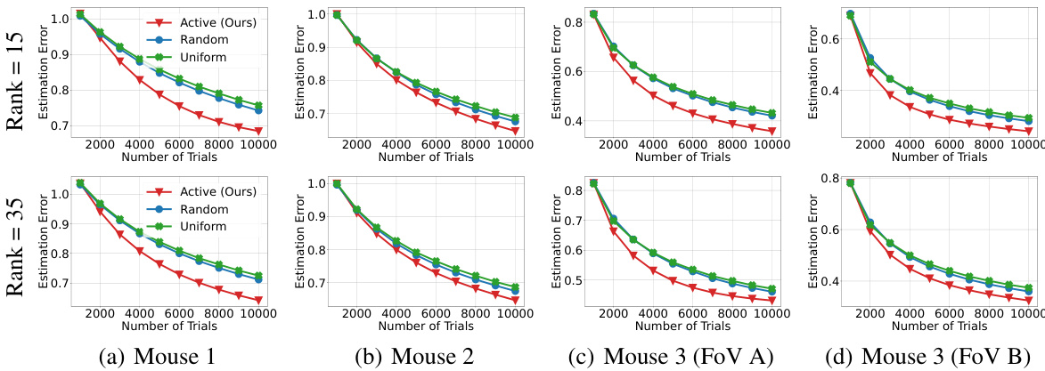
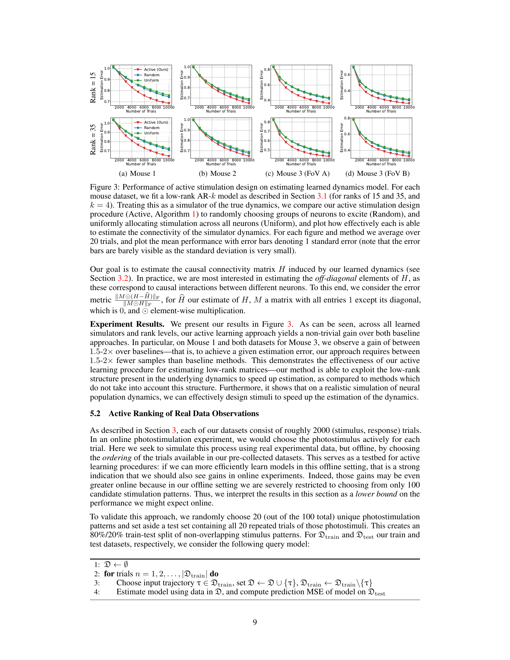
This figure compares three different methods for estimating the connectivity matrix of a learned dynamical system: Active (the authors’ proposed method), Random (randomly choosing neurons to stimulate), and Uniform (uniformly stimulating all neurons). The results show that the Active method outperforms the other two methods in terms of estimation accuracy. The performance is averaged over 20 trials, with error bars indicating the standard error.
This figure compares three different methods for estimating the connectivity matrix of a learned neural population dynamics model: active stimulation design, random stimulation, and uniform stimulation. The results show that the active learning method outperforms the other two, achieving a given estimation error with significantly fewer trials. The results are shown for four different mouse datasets, with separate plots for low-rank models of rank 15 and 35.

This figure demonstrates the predictive performance of low-rank autoregressive (AR) models and gated recurrent unit (GRU) networks on neural population activity data. It shows roll-out predictions of neural activity, receiver operating characteristic (ROC) curves, area under the ROC curve (AUROC) and mean squared error (MSE) for different model ranks, illustrating the effectiveness of low-rank models in capturing the dynamics of neural populations. The figure also highlights the distinction between direct and indirect stimulation effects on neural activity.
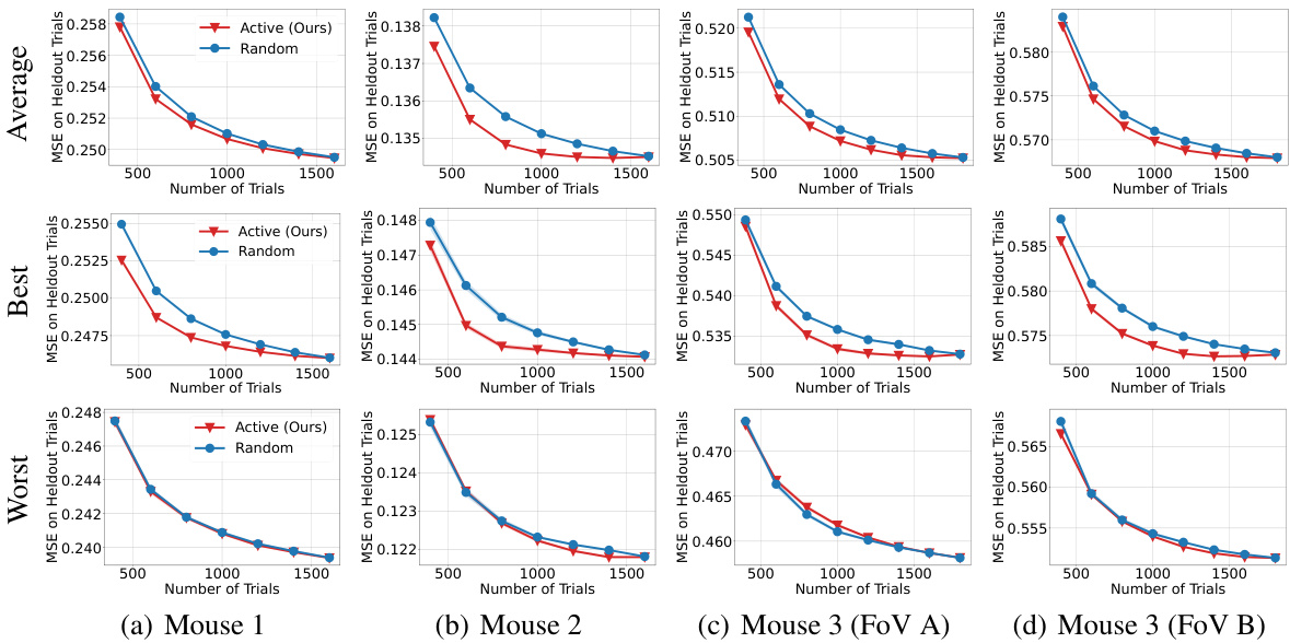
This figure demonstrates the predictive performance of low-rank Autoregressive (AR) models and Gated Recurrent Unit (GRU) networks on neural population activity data. It shows example roll-out predictions of neural activity, receiver operating characteristic (ROC) curves for response detection, and mean square error (MSE) values. The results suggest that low-rank AR models provide a good balance between predictive accuracy and model complexity.

This figure compares the estimated and true neural activity for three neurons (0, 3, and 95) in Mouse 2 across different levels of mean squared error (MSE) on held-out trials. The MSE values represent the model’s predictive accuracy on unseen data, with lower MSE indicating better performance. Each subplot shows the comparison for a specific neuron and MSE level, illustrating how well the model’s predictions match the actual recorded neural activity.

This figure compares the estimated neural activity with the true neural activity for three different neurons (0, 3, and 95) in Mouse 2 at four different levels of mean squared error (MSE) on held-out trials. Each subplot shows the true and estimated activity over time, illustrating the model’s performance at different accuracy levels. The overall MSE values reflect how well the model predicts the neural activity on unseen data.

This figure shows the comparison between estimated and true neural activity for three neurons (0, 3, and 95) in Mouse 2 at various levels of mean squared error (MSE). Each subplot represents a neuron and displays the true activity (blue) and the estimated activity (orange) over time. The MSE value for each subplot indicates the prediction accuracy of the model. This visualization helps illustrate the model’s ability to predict neural activity with varying degrees of accuracy based on the overall MSE of the model, providing a detailed evaluation of the model’s performance.
Full paper#
