TL;DR#
Deep learning models are computationally expensive, creating challenges for deployment on resource-limited devices. Existing adaptive depth networks that adjust model depth to match resource availability are often complex and time-consuming to train. This research addresses these issues by presenting a novel method for building adaptive-depth networks that drastically reduces the training time. The core of the method is dividing each residual stage of a network into two paths - a mandatory path for core feature learning and a skippable path for refinement. A self-distillation strategy is used to train these paths, where the skippable path is optimized to minimize performance degradation when skipped. This allows the network to efficiently select various depths at testing time without needing to retrain.
The approach achieves this by applying a self-distillation technique. The largest and smallest networks are used as teacher and student, respectively. Instead of retraining each sub-network, this strategy significantly reduces training time. At testing time, the network can select different depths by combinatorially selecting which sub-paths to use. This allows selection of sub-networks with various accuracy-efficiency trade-offs from a single model. The paper demonstrates the method’s effectiveness on several deep learning models, including CNNs and transformers, showing improved performance compared to traditional approaches. This work provides an architectural pattern and training strategy generally applicable to various network architectures. It also delivers a theoretical foundation explaining why this method can reduce errors and minimize the impact of skipping sub-paths.
Key Takeaways#
Why does it matter?#
This paper is important because it introduces a novel and efficient approach to adaptive depth networks, a crucial area in optimizing deep learning models for various resource constraints. The proposed method offers a significant reduction in training time compared to existing methods, while still achieving comparable or better performance. This opens new avenues for research in developing more efficient and adaptable deep learning models, particularly relevant to the growing demand for deploying such models on resource-limited devices. The formal analysis provided offers valuable theoretical insights for further development in the field. The open-source code release further enhances the impact by fostering wider adoption and future work building upon their contributions.
Visual Insights#

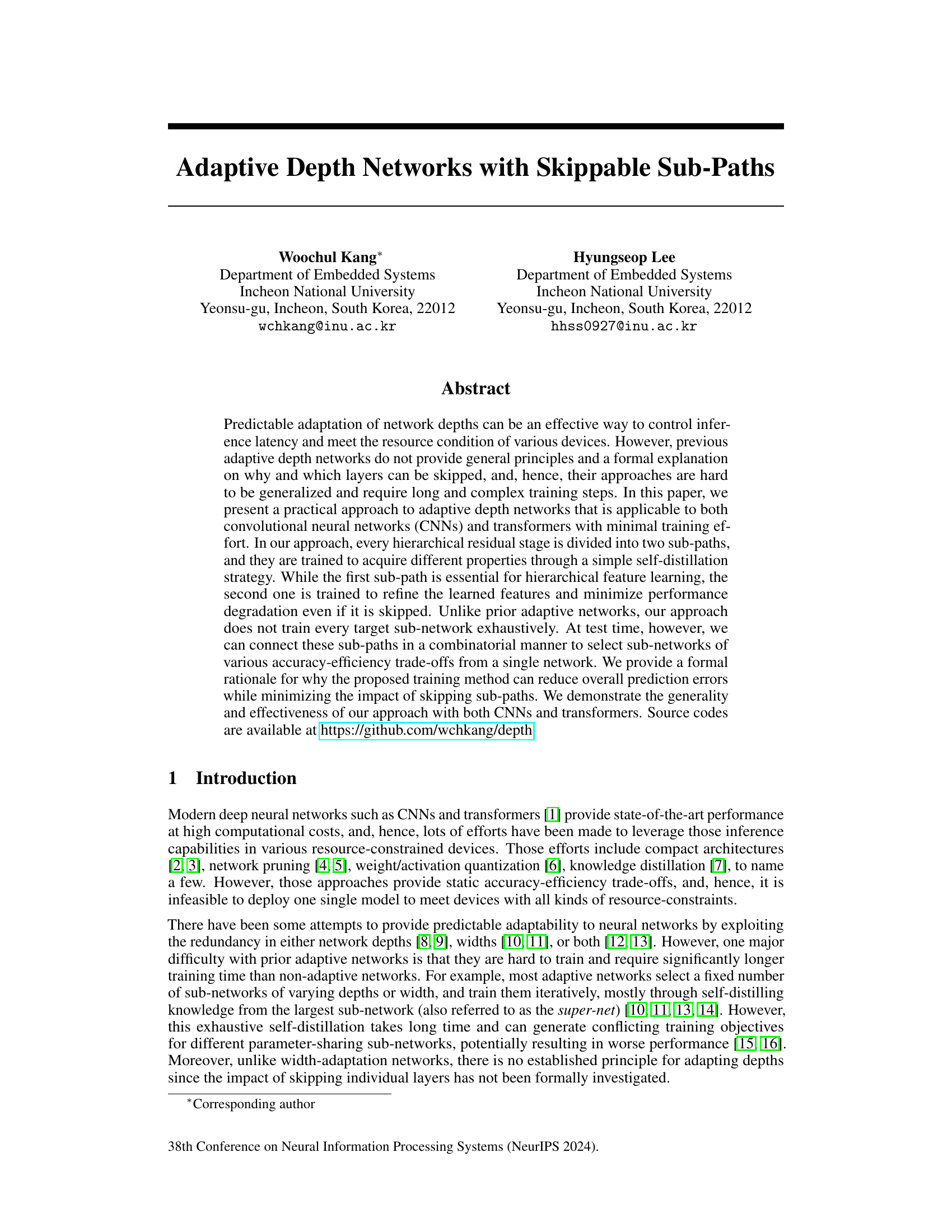
🔼 This figure illustrates the training and testing process of the proposed adaptive depth networks. During training, each residual stage is split into two sub-paths: a mandatory path and a skippable path. The skippable paths are trained using a self-distillation strategy to minimize performance loss when skipped. During testing, these skippable paths can be selectively skipped, creating a range of sub-networks with varying accuracy and efficiency. The resulting Pareto frontier of these sub-networks surpasses that achievable by training individual networks separately.
read the caption
Figure 1: (a) During training, every residual stage of a network is divided into two sub-paths. The layers in every second (orange) sub-path are optimized to minimize performance degradation even if they are skipped. (b) At test time, these second sub-paths can be skipped in a combinatorial manner, allowing instant selection of various parameter sharing sub-networks. (c) The sub-networks selected from a single network form a better Pareto frontier than counterpart individual networks.
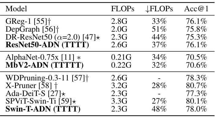
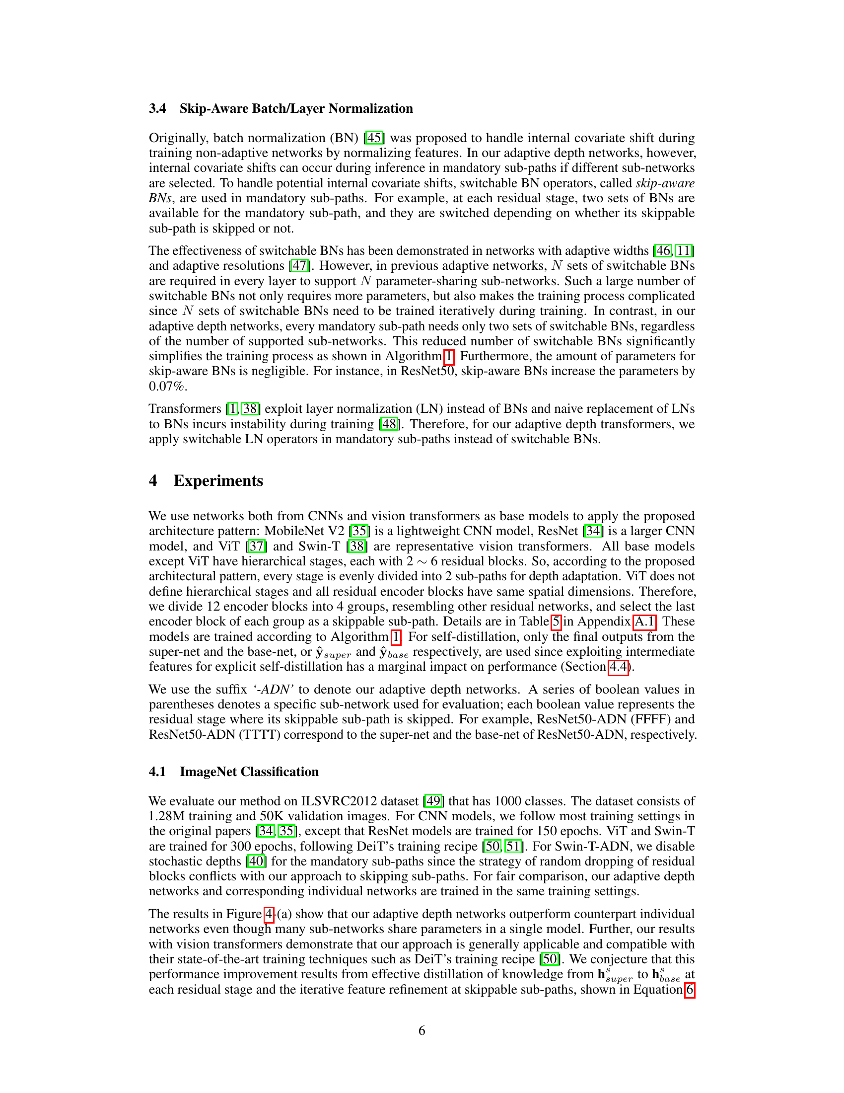
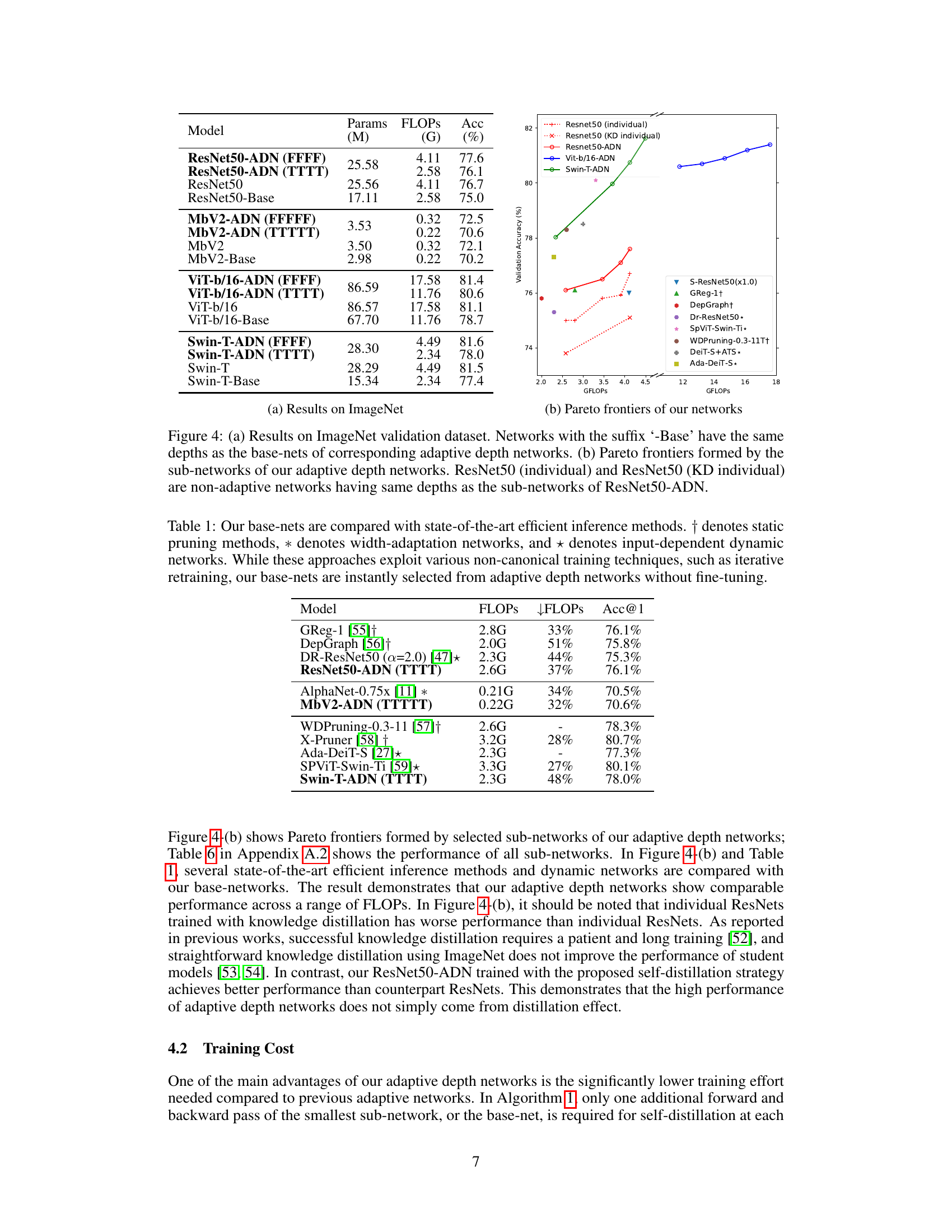
🔼 This table compares the performance of the base networks (smallest sub-networks) of the proposed adaptive depth networks against other state-of-the-art efficient inference methods. It highlights that the base networks, selected directly without further fine-tuning, achieve competitive accuracy while using fewer FLOPs. The table emphasizes that unlike other methods which might use techniques like iterative retraining, the base networks are directly selected, showcasing the efficiency of the proposed approach.
read the caption
Table 1: Our base-nets are compared with state-of-the-art efficient inference methods. † denotes static pruning methods, * denotes width-adaptation networks, and * denotes input-dependent dynamic networks. While these approaches exploit various non-canonical training techniques, such as iterative retraining, our base-nets are instantly selected from adaptive depth networks without fine-tuning.
In-depth insights#
Adaptive Depth Nets#
Adaptive depth networks represent a significant advancement in neural network efficiency. By strategically enabling the skipping of certain layers during inference, latency and computational costs are reduced without severely compromising accuracy. This adaptability is achieved through a novel training approach that divides each residual stage into two sub-paths: a mandatory path crucial for feature learning and a skippable path designed for refinement. A key innovation is the self-distillation strategy, which trains these sub-paths to minimize performance degradation even when skipped, eliminating the need for exhaustive training of all possible sub-networks. The resulting single network can dynamically adapt to various resource constraints at test time, providing a superior accuracy-efficiency trade-off compared to traditional static networks. The formal analysis provided further solidifies the theoretical foundation of this adaptive technique, demonstrating its efficacy in reducing prediction errors while maintaining feature representation quality.
Self-Distillation#
The concept of self-distillation in this research paper centers on training sub-networks within a larger network to minimize performance degradation when certain layers are skipped. This is achieved by using a self-supervised learning strategy where the largest and smallest sub-networks (super-net and base-net) act as teacher and student respectively, ensuring efficient transfer of knowledge without exhaustive training of every potential sub-network. This approach is particularly effective due to its simplicity and ability to reduce training time. The core idea revolves around optimizing skippable sub-paths to preserve feature level information, essentially mimicking the properties of residual blocks and refining features without significantly altering the input. This method is shown to improve prediction accuracy and resource efficiency, while offering a more general and robust approach to adaptive depth networks compared to prior methods.
Skippable Subpaths#
The concept of “Skippable Subpaths” introduces a novel approach to adaptive depth networks. The core idea revolves around dividing each hierarchical residual stage into two distinct sub-paths: a mandatory path essential for hierarchical feature learning and a skippable path designed to refine features while minimizing performance degradation if skipped. This architecture enables efficient inference by dynamically selecting sub-networks with various accuracy-latency trade-offs at test time through combinatorial activation of the sub-paths. A crucial aspect is the training strategy that utilizes self-distillation to optimize the skippable paths to preserve the essential feature distributions even when skipped, which reduces overall prediction errors while avoiding exhaustive sub-network training. The formal analysis provided supports the effectiveness of this technique by demonstrating that the residual functions in the skippable paths reduce errors iteratively without significantly altering feature distributions. This approach enhances both the efficiency and adaptability of deep networks.
Formal Analysis#
The heading ‘Formal Analysis’ suggests a section dedicated to mathematically rigorous justification of the proposed method. It likely delves into the theoretical underpinnings of the adaptive depth network’s efficiency, specifically addressing why skipping certain sub-paths during inference doesn’t significantly impact performance. This involves demonstrating that the trained skippable sub-paths primarily act as feature refinement units, making minimal alterations to the overall feature representation. Taylor expansion might be used to approximate the loss function, showing that the impact of skipping these paths is minimal. The analysis would likely provide a formal guarantee, establishing a connection between the training methodology and the reduced prediction error even with fewer layers. Crucially, the formal analysis would aim to prove that the trained model behaves as intended and isn’t merely an empirical observation. The ultimate goal is to provide a mathematical foundation explaining the success of their proposed architecture.
On-device Efficiency#
On-device efficiency is a crucial aspect of deploying deep learning models, especially in resource-constrained environments. The paper likely investigates methods to optimize model inference for reduced latency and energy consumption. This could involve techniques like model compression, quantization, or adaptive computation. The results section probably showcases a comparison of the proposed approach against existing techniques, highlighting improvements in terms of speed and power efficiency. A key consideration is the trade-off between accuracy and efficiency; the paper would likely demonstrate that the proposed methods maintain reasonable accuracy despite the optimizations. Therefore, the focus is on practical deployment, showing how improvements translate to real-world benefits on target devices, particularly concerning power usage and inference time.
More visual insights#
More on figures

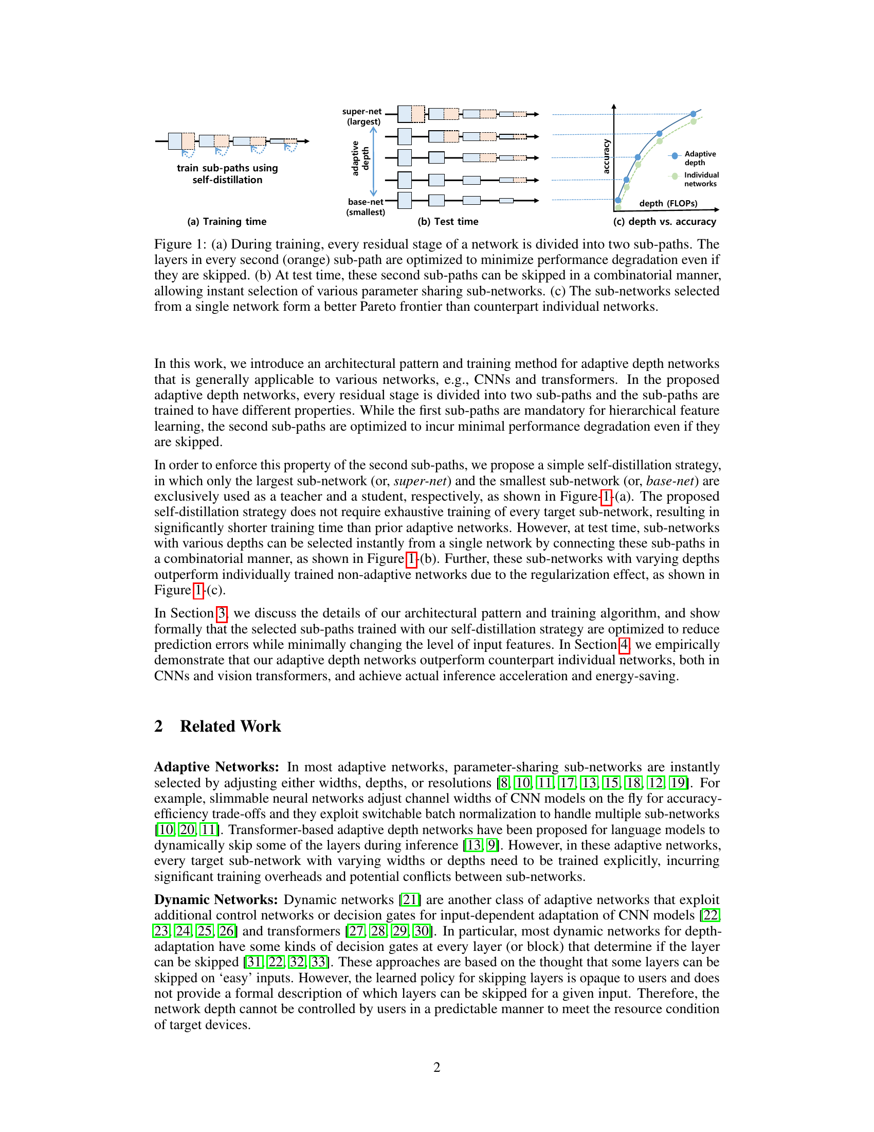
🔼 This figure illustrates a residual stage divided into two sub-paths: a mandatory path (blue) essential for hierarchical feature learning, and a skippable path (orange) trained to minimize performance degradation if skipped. The skippable path is trained using self-distillation to maintain similar feature distributions compared to the mandatory path. At test time, the skippable path can be skipped or not, enabling various sub-network configurations.
read the caption
Figure 2: Illustration of a residual stage with two sub-paths. While the first (blue) sub-path is mandatory for hierarchical feature learning, the second (orange) sub-path can be skipped for efficiency. The layers in the skippable sub-path are trained to preserve the feature distribution from hbase to hsuper using the proposed self-distillation strategy. Having similar distributions, either hbase or hsuper can be provided as input h to the next residual stage. In the mandatory sub-path, another set of batch normalization operators, called skip-aware BNs, is exploited if the second sub-path is skipped. These sub-paths are building blocks to construct sub-networks of varying depths.

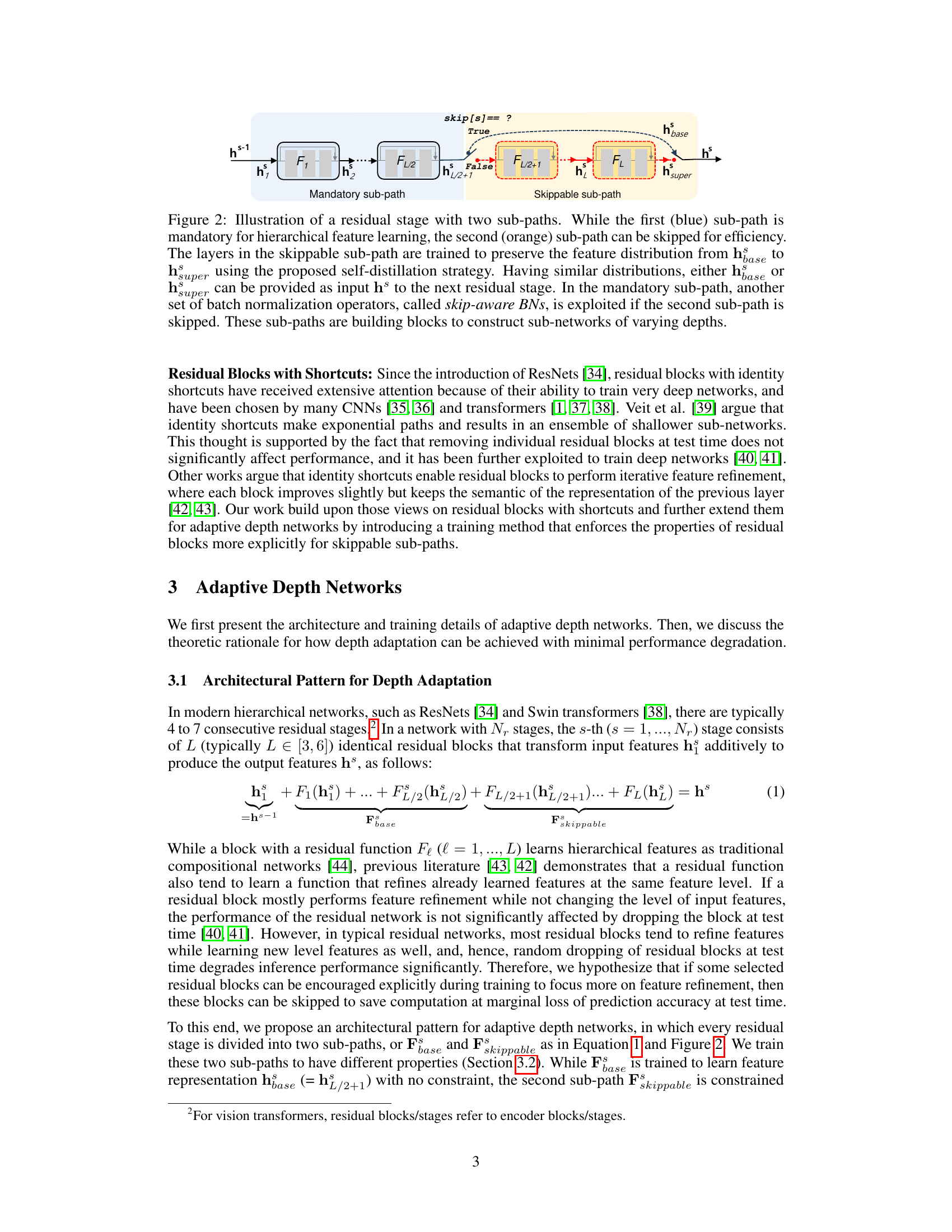
🔼 This figure compares the magnitude of transformation done by each residual block in ResNet50 and ResNet50-ADN. ResNet50-ADN is the adaptive depth network proposed in the paper. The y-axis shows ||F(h)||2/||h||2, which represents the magnitude of transformation performed by each residual block (F) relative to the input (h). The x-axis represents the index of the residual blocks, grouped by stage. The figure demonstrates that the skippable sub-paths in ResNet50-ADN (orange regions) have much smaller transformation magnitudes compared to ResNet50, indicating that they primarily refine features instead of learning new features, as intended by the self-distillation training strategy.
read the caption
Figure 3: ||F(h)||2/||h||2 at residual blocks.
🔼 This figure illustrates the training and testing phases of the proposed adaptive depth networks. During training (a), each residual stage is split into two sub-paths: a mandatory path crucial for feature learning and a skippable path trained to minimize performance loss if skipped. The skippable paths use self-distillation. During testing (b), these skippable paths can be selectively skipped to create various sub-networks with different accuracy-efficiency trade-offs, all stemming from a single trained network. Finally, (c) shows that the resulting sub-networks achieve superior performance compared to training individual networks.
read the caption
Figure 1: (a) During training, every residual stage of a network is divided into two sub-paths. The layers in every second (orange) sub-path are optimized to minimize performance degradation even if they are skipped. (b) At test time, these second sub-paths can be skipped in a combinatorial manner, allowing instant selection of various parameter sharing sub-networks. (c) The sub-networks selected from a single network form a better Pareto frontier than counterpart individual networks.
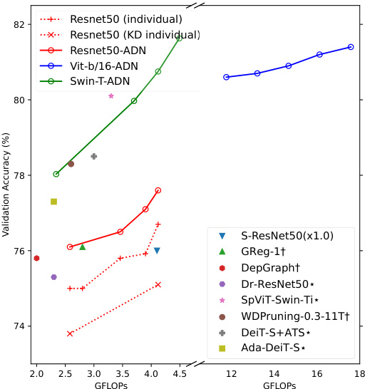
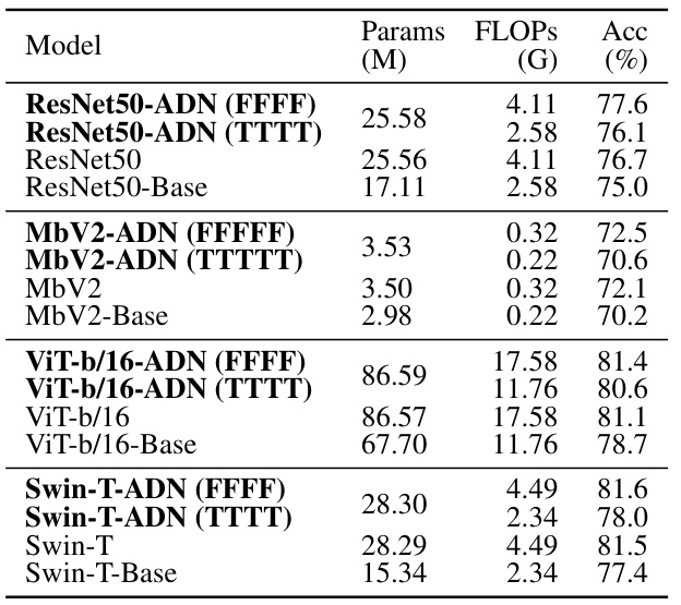
🔼 This figure presents the ImageNet validation accuracy results for various networks, including the proposed adaptive depth networks. Panel (a) compares the accuracy of the proposed adaptive depth networks (with different depths selected at test time) to individually trained networks with fixed depths. The suffix ‘-Base’ in the network names indicates that these networks have the same depth as the smallest sub-network in the corresponding adaptive depth network. Panel (b) shows Pareto frontiers, illustrating the accuracy-efficiency trade-offs achievable by selecting various sub-networks from a single trained adaptive depth network. The Pareto frontier for the adaptive depth networks dominates those of individually trained networks, showing the superiority of the proposed approach.
read the caption
Figure 4: (a) Results on ImageNet validation dataset. Networks with the suffix '-Base' have the same depths as the base-nets of corresponding adaptive depth networks. (b) Pareto frontiers formed by the sub-networks of our adaptive depth networks. ResNet50 (individual) and ResNet50 (KD individual) are non-adaptive networks having same depths as the sub-networks of ResNet50-ADN.

🔼 This figure shows the validation accuracy curves during training for several sub-networks of ResNet50-ADN and Swin-T-ADN. Each line represents a sub-network with a different depth, indicated by the combination of ‘F’ (full sub-path) and ‘T’ (truncated sub-path) for each residual stage. The key takeaway is that, although only the largest and smallest networks were explicitly trained, many other intermediate-depth networks achieve high accuracy because the training methodology allows them to readily adapt depth at test time. The consistent increase in validation accuracy for many of the networks shows that depth adaptation provides a performance boost.
read the caption
Figure 5: Validation accuracy of sub-networks of our adaptive depth networks during training. Many sub-networks of varying depths become available from a single network even though most of them are not explicitly trained.
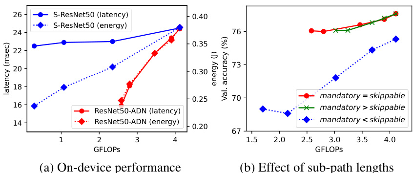
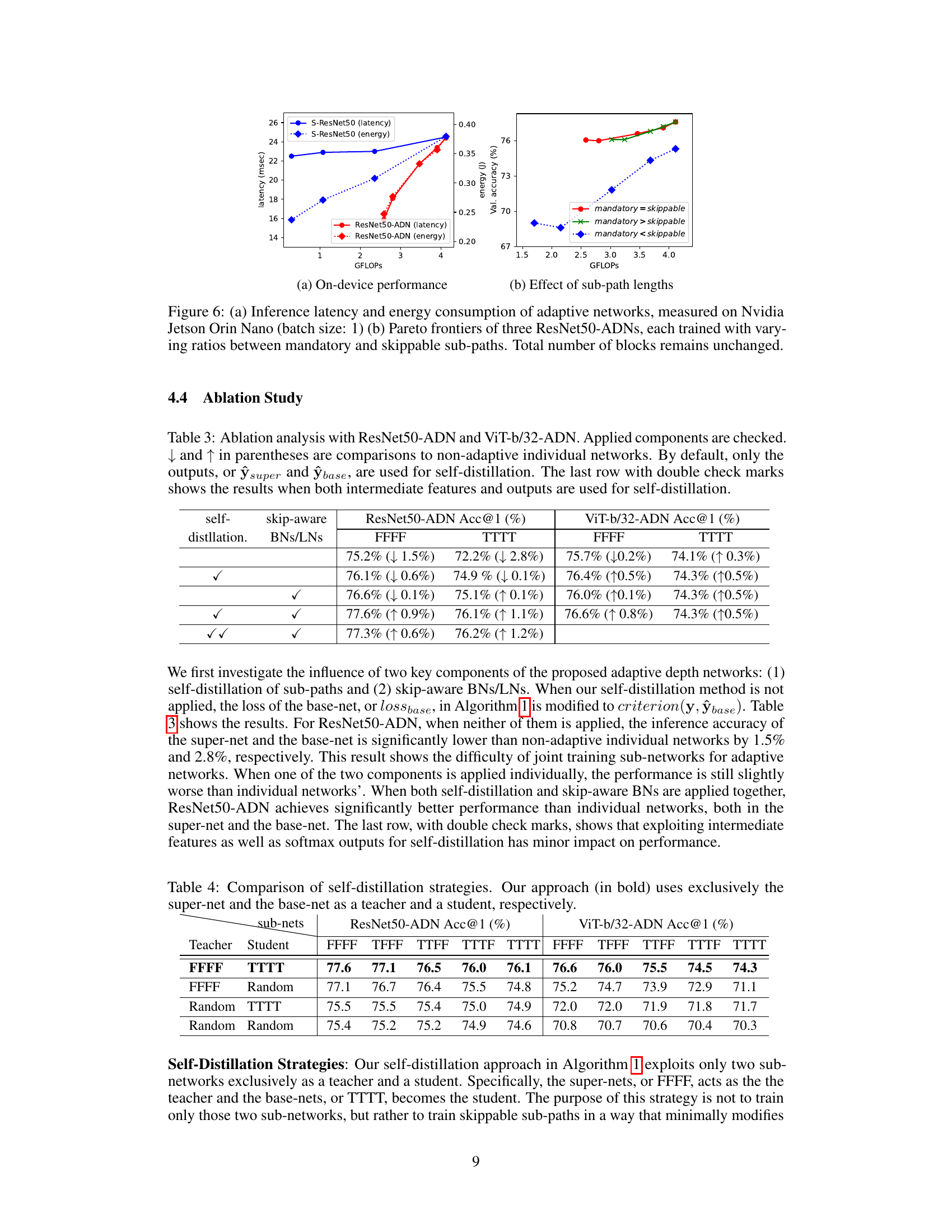
🔼 This figure shows the results of inference latency and energy consumption of ResNet50-ADN on Nvidia Jetson Orin Nano and compares it with S-ResNet50. The results indicate that depth adaptation is very effective in accelerating inference speed and reducing energy consumption. It also shows the Pareto frontier of three different ResNet50-ADNs each trained with different ratios between the mandatory and skippable sub-paths. This demonstrates the effect of the sub-path lengths on performance.
read the caption
Figure 6: (a) Inference latency and energy consumption of adaptive networks, measured on Nvidia Jetson Orin Nano (batch size: 1) (b) Pareto frontiers of three ResNet50-ADNs, each trained with varying ratios between mandatory and skippable sub-paths. Total number of blocks remains unchanged.
🔼 This figure illustrates the training and testing procedures of the proposed adaptive depth networks. Panel (a) shows how each residual stage is split into two sub-paths during training: a mandatory path (blue) essential for feature learning, and a skippable path (orange) trained to minimize performance loss if skipped. Panel (b) demonstrates how, at test time, these skippable paths can be selectively excluded to create a range of sub-networks with different computational costs and accuracies. Finally, panel (c) shows that these dynamically generated sub-networks outperform individually trained networks of comparable size in terms of accuracy/efficiency trade-off.
read the caption
Figure 1: (a) During training, every residual stage of a network is divided into two sub-paths. The layers in every second (orange) sub-path are optimized to minimize performance degradation even if they are skipped. (b) At test time, these second sub-paths can be skipped in a combinatorial manner, allowing instant selection of various parameter sharing sub-networks. (c) The sub-networks selected from a single network form a better Pareto frontier than counterpart individual networks.

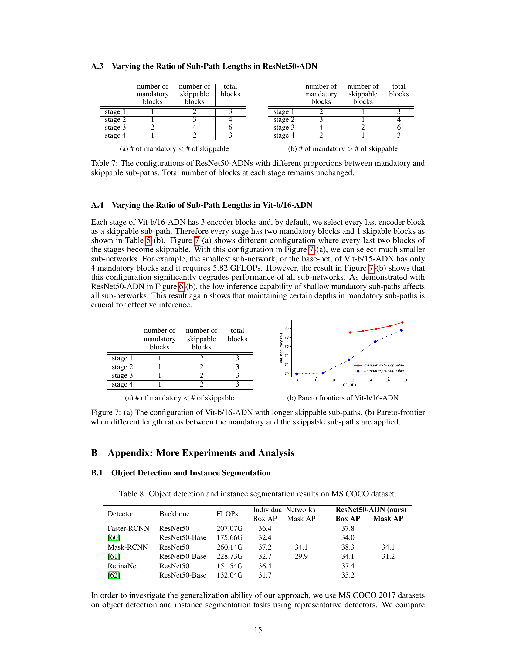
🔼 Figure 7(a) shows a modified configuration of Vit-b/16-ADN where every last two blocks of the stages are skippable instead of only the last block. This allows for selecting much smaller sub-networks. Figure 7(b) shows the Pareto frontier of this modified Vit-b/16-ADN configuration as well as configurations with varying ratios of mandatory to skippable sub-paths. The results show that maintaining certain depths in mandatory sub-paths is crucial for effective inference.
read the caption
Figure 7: (a) The configuration of Vit-b/16-ADN with longer skippable sub-paths. (b) Pareto-frontier when different length ratios between the mandatory and the skippable sub-paths are applied.

🔼 Figure 6(a) compares the inference latency and energy consumption of ResNet50-ADN and S-ResNet50 on Nvidia Jetson Orin Nano. The results show that the depth-adaptation in ResNet50-ADN is effective in accelerating inference speed and reducing energy consumption, while the width-adaptation in S-ResNet50 achieves only a limited speedup. Figure 6(b) shows Pareto frontiers formed by sub-networks of three ResNet50-ADNs, each having different ratio between mandatory and skippable sub-paths, demonstrating the effect of varying the ratio of sub-path lengths on the performance.
read the caption
Figure 6: (a) Inference latency and energy consumption of adaptive networks, measured on Nvidia Jetson Orin Nano (batch size: 1) (b) Pareto frontiers of three ResNet50-ADNs, each trained with varying ratios between mandatory and skippable sub-paths. Total number of blocks remains unchanged.

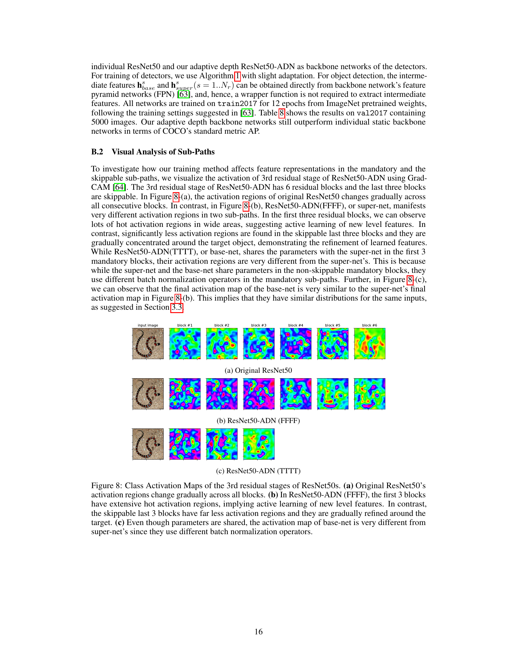
🔼 This figure visualizes the activation maps of the 3rd residual stage in ResNet50 and ResNet50-ADN using Grad-CAM. It shows how the activation regions change across the blocks in both networks. In the original ResNet50, the activation regions change gradually. However, in ResNet50-ADN, the first three blocks (mandatory path) show extensive activation, indicating new feature learning, while the last three blocks (skippable path) show concentrated activation around the target object, indicating refinement of learned features. Even though the mandatory blocks share parameters between the super-net and base-net, their activation maps differ due to the use of different batch normalization operators.
read the caption
Figure 8: Class Activation Maps of the 3rd residual stages of ResNet50s. (a) Original ResNet50's activation regions change gradually across all blocks. (b) In ResNet50-ADN (FFFF), the first 3 blocks have extensive hot activation regions, implying active learning of new level features. In contrast, the skippable last 3 blocks have far less activation regions and they are gradually refined around the target. (c) Even though parameters are shared, the activation map of base-net is very different from super-net's since they use different batch normalization operators.
More on tables
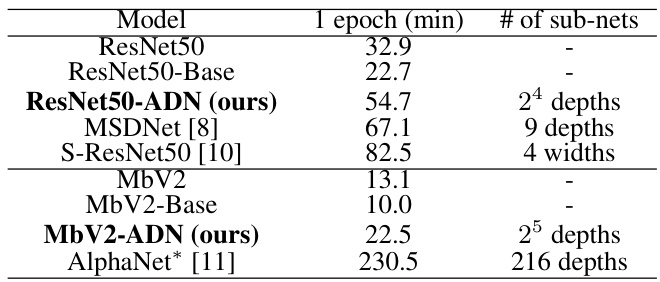
🔼 This table compares the training time for one epoch of different adaptive depth networks and non-adaptive counterparts, including ResNet50, MbV2, and their baselines. It also includes the number of sub-networks considered for each model. The training time is measured using an Nvidia RTX 4090 GPU with a batch size of 128. AlphaNet is included for comparison, but it is configured differently to focus on depth adaptation alone.
read the caption
Table 2: Training time (1 epoch), measured on Nvidia RTX 4090 (batch size: 128). AlphaNet* is configured to have similar FLOPs to MbV2 and only adjusts its depth to select sub-networks.

🔼 This table presents the ablation study results for ResNet50-ADN and ViT-b/32-ADN, demonstrating the impact of self-distillation and skip-aware batch/layer normalization on the models’ performance. The table shows that both techniques are beneficial, and that the combination of the two yields the best results. The last row shows the marginal impact of including intermediate features in self-distillation.
read the caption
Table 3: Ablation analysis with ResNet50-ADN and ViT-b/32-ADN. Applied components are checked. ↓ and ↑ in parentheses are comparisons to non-adaptive individual networks. By default, only the outputs, or ŷ super and ŷbase, are used for self-distillation. The last row with double check marks shows the results when both intermediate features and outputs are used for self-distillation.

🔼 This table compares different self-distillation strategies used to train the adaptive depth networks. The standard approach uses the largest network (super-net) and the smallest network (base-net) exclusively as teacher and student. Other rows explore random sampling of networks for teacher/student roles in the self-distillation process. The results demonstrate that the proposed approach, using super-net and base-net exclusively, outperforms the random sampling strategies for both ResNet50-ADN and ViT-b/32-ADN networks.
read the caption
Table 4: Comparison of self-distillation strategies. Our approach (in bold) uses exclusively the super-net and the base-net as a teacher and a student, respectively.

🔼 This table shows the architecture details of the adaptive depth networks used in the experiments. It breaks down the number of mandatory and skippable blocks in each stage for four different network models: ResNet50-ADN, ViT-b/16-ADN, MbV2-ADN, and Swin-T-ADN. Note that ViT, unlike the others, doesn’t have inherent hierarchical stages, so its 12 encoder blocks are grouped into 4 stages for consistency.
read the caption
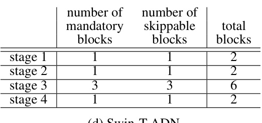
Table 5: Each stage of base models is evenly divided into two sub-paths; the first is mandatory and the other is skippable. Since ViT does not define hierarchical stages, 12 identical encoder blocks are divided into 4 stages, resembling other residual networks for vision tasks.

🔼 This table details the architecture of four different network models (ResNet50-ADN, ViT-b/16-ADN, MbV2-ADN, and Swin-T-ADN) showing how each stage is divided into mandatory and skippable blocks. It highlights that while most models have hierarchical stages, ViT (Vision Transformer) is treated differently due to its lack of explicit hierarchical stages. The table provides a clear picture of the division of blocks for each stage in the adaptive depth networks.
read the caption
Table 5: Each stage of base models is evenly divided into two sub-paths; the first is mandatory and the other is skippable. Since ViT does not define hierarchical stages, 12 identical encoder blocks are divided into 4 stages, resembling other residual networks for vision tasks.
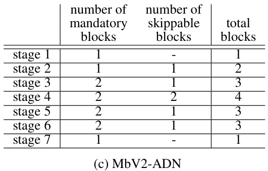
🔼 This table details the architecture of the adaptive depth networks used in the paper. It shows how each stage in different network models (ResNet50-ADN, ViT-b/16-ADN, MbV2-ADN, Swin-T-ADN) is divided into mandatory and skippable sub-paths (blocks). For the Vision Transformer (ViT), the 12 encoder blocks are grouped into four stages to mimic the hierarchical structure of the other network types.
read the caption
Table 5: Each stage of base models is evenly divided into two sub-paths; the first is mandatory and the other is skippable. Since ViT does not define hierarchical stages, 12 identical encoder blocks are divided into 4 stages, resembling other residual networks for vision tasks.
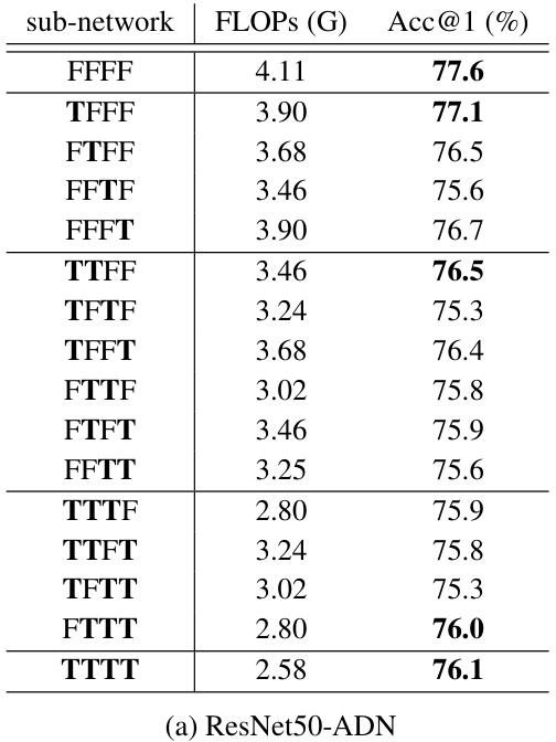
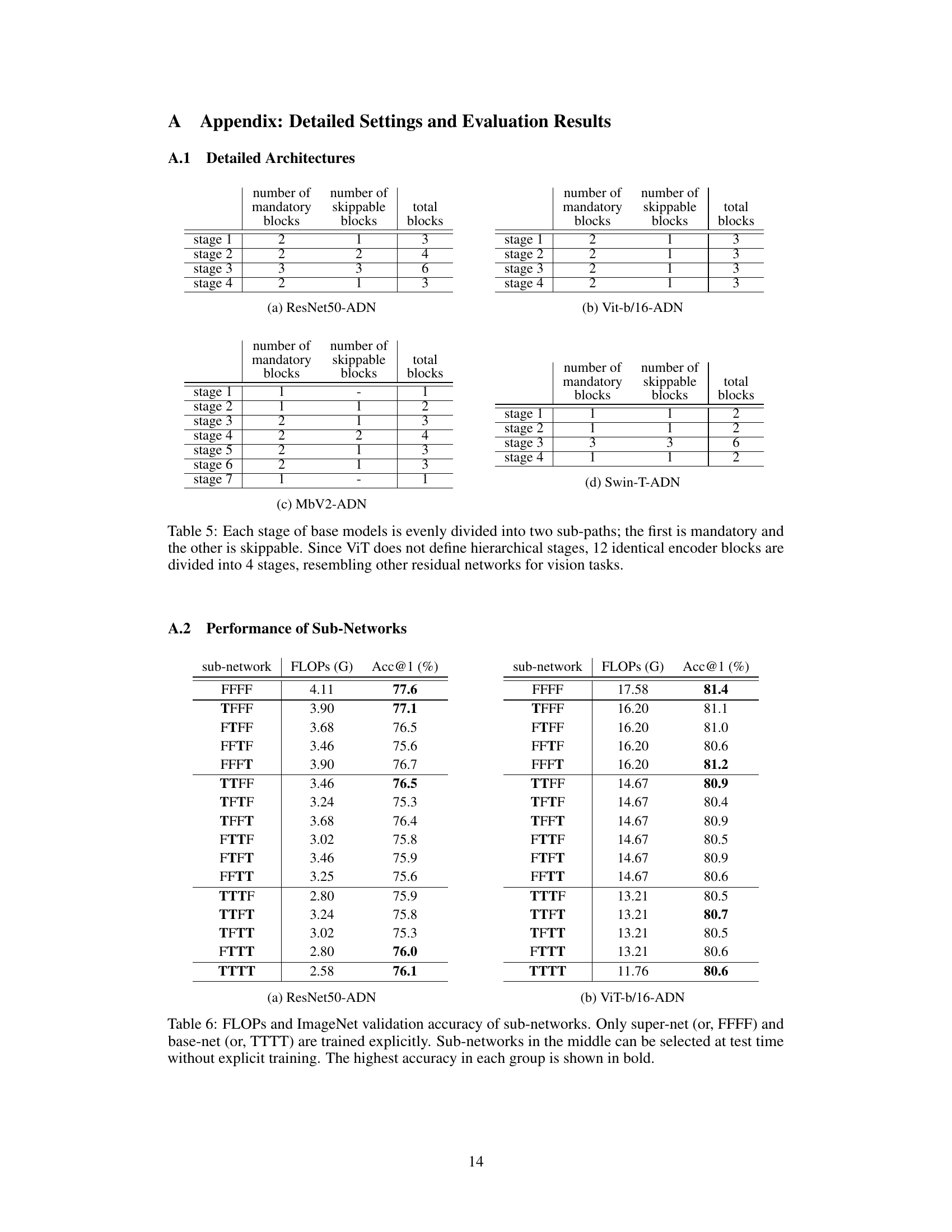
🔼 This table presents the performance of various sub-networks derived from a single ResNet50-ADN model. Each row shows a specific sub-network configuration, denoted by a string of ‘F’s (for including the skippable sub-path) and ‘T’s (for skipping the sub-path) corresponding to each residual stage. The FLOPs (in GigaFLOPS) and the accuracy (in %) on the ImageNet validation set are reported for each sub-network. Only the largest (FFFF) and smallest (TTTT) sub-networks are trained explicitly; the intermediate sub-networks’ performance are evaluated without explicit training.
read the caption
Table 6: FLOPs and ImageNet validation accuracy of sub-networks. Only super-net (or, FFFF) and base-net (or, TTTT) are trained explicitly. Sub-networks in the middle can be selected at test time without explicit training. The highest accuracy in each group is shown in bold.

🔼 This table presents the performance of various sub-networks derived from a single adaptive depth network. Each row represents a different sub-network configuration, indicated by a sequence of ‘F’ (for the skippable sub-path not skipped) or ‘T’ (for the skippable sub-path skipped) for each of the residual stages. The table shows the FLOPs (floating-point operations) and the accuracy on the ImageNet validation dataset for each configuration. Only the largest (‘FFFF’) and smallest (‘TTTT’) sub-networks are explicitly trained; the other sub-networks are evaluated without explicit training, demonstrating the efficiency of the approach.
read the caption
Table 6: FLOPs and ImageNet validation accuracy of sub-networks. Only super-net (or, FFFF) and base-net (or, TTTT) are trained explicitly. Sub-networks in the middle can be selected at test time without explicit training. The highest accuracy in each group is shown in bold.
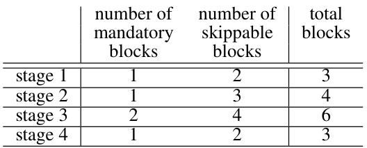
🔼 This table shows different configurations of ResNet50-ADNs by varying the ratio of mandatory and skippable sub-paths within each stage. While the total number of blocks per stage remains constant across all configurations, the distribution between mandatory and skippable blocks changes. This allows for an exploration of how different ratios impact the overall network performance.
read the caption
Table 7: The configurations of ResNet50-ADNs with different proportions between mandatory and skippable sub-paths. Total number of blocks at each stage remains unchanged.

🔼 This table shows the architecture of the four different models used in the paper. Each stage of the model is divided into mandatory and skippable sub-paths. The table also notes that the Vision Transformer (ViT) model does not have hierarchical stages, so 12 encoder blocks are divided into 4 stages.
read the caption
Table 5: Each stage of base models is evenly divided into two sub-paths; the first is mandatory and the other is skippable. Since ViT does not define hierarchical stages, 12 identical encoder blocks are divided into 4 stages, resembling other residual networks for vision tasks.

🔼 This table compares the performance of different object detectors (Faster-RCNN, Mask-RCNN, RetinaNet) using ResNet50 and ResNet50-Base (the base network of ResNet50-ADN) as backbones. It shows the Box AP (Average Precision for bounding boxes) and Mask AP (Average Precision for masks) for each detector and backbone, demonstrating the improvement in performance achieved using the adaptive depth network (ResNet50-ADN).
read the caption
Table 8: Object detection and instance segmentation results on MS COCO dataset.
Full paper#
