↗ OpenReview ↗ NeurIPS Homepage ↗ Chat
TL;DR#
Partial differential equations (PDEs) are fundamental in science and engineering. Forecasting and data assimilation are crucial tasks, but existing numerical and machine learning methods often fall short, particularly when integrating sparse observations. This necessitates more robust and accurate models, capable of handling both prediction and assimilation. Diffusion models, known for their conditional generation capabilities, show promise for overcoming these challenges.
This research enhances score-based diffusion models to better suit forecasting and assimilation. Three key innovations are introduced: 1) an autoregressive sampling method that drastically improves forecasting accuracy; 2) a novel training technique resulting in more robust and stable performance over different history lengths; and 3) a hybrid model that combines pre-training on initial conditions with post-training conditioning, making it highly flexible in handling various data assimilation scenarios. Empirical evaluations show that these improvements are crucial for tackling combined forecasting and data assimilation, common in real-world applications.
Key Takeaways#
Why does it matter?#
This paper is crucial for researchers in PDE modeling and data assimilation. It presents novel methods to improve forecasting and data assimilation accuracy using diffusion models, addressing limitations of previous approaches. This opens avenues for more accurate predictions and better integration of observations in various scientific and engineering domains.
Visual Insights#

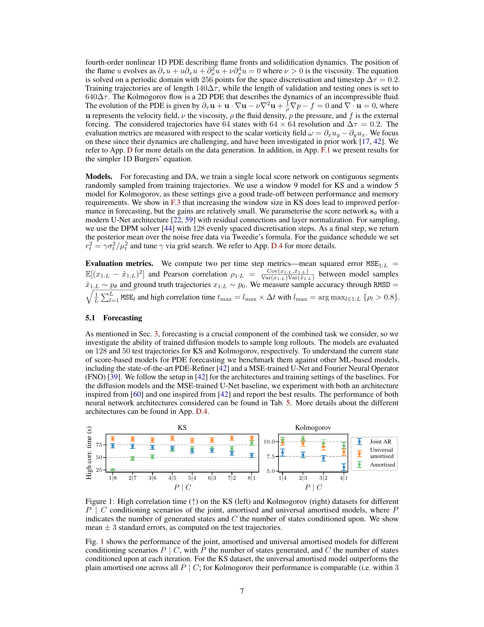
This figure compares the forecasting performance of three different diffusion models (Joint AR, Amortised, and Universal Amortised) on the Kuramoto-Sivashinsky (KS) and Kolmogorov datasets. The x-axis shows different conditioning scenarios represented as P|C, where P is the number of generated states and C is the number of conditioning states. The y-axis represents the high correlation time, a metric indicating the model’s ability to generate accurate and long-range forecasts. Error bars show mean ± 3 standard errors across the test trajectories, indicating the variability in the results. The figure demonstrates that the models’ performance varies across different conditioning scenarios and datasets.

The table compares three different score-based diffusion models used in the paper for forecasting and data assimilation tasks. It categorizes them based on three key characteristics: the type of score network (joint or conditional, indicating whether it is trained on the full joint distribution or conditioned on some observations), the rollout strategy used during sampling (all-at-once or autoregressive), and how conditioning is handled during inference (guidance or architectural).
In-depth insights#
Conditional Diffusion#
Conditional diffusion models represent a powerful advancement in generative modeling, particularly for their ability to incorporate conditioning information effectively. They elegantly blend the flexibility of diffusion models with the control offered by conditional approaches. This allows for the generation of samples that adhere to specific constraints or exhibit desired characteristics. The core idea lies in modifying the diffusion process itself to incorporate conditions, whether during the forward diffusion process (adding condition to the noise schedule) or during the reverse diffusion process (by guiding the denoising trajectory toward desired features). A key advantage lies in their capacity to handle various types of conditioning, ranging from simple labels to complex data points, even high-dimensional ones. However, the increased complexity compared to unconditional diffusion models brings challenges, including increased computational cost and potential instabilities during training when conditioning is improperly implemented. Furthermore, the impact of conditioning on the model’s ability to generate diverse and high-quality outputs needs careful consideration and empirical evaluation, highlighting the importance of choosing appropriate architectures and training techniques to effectively leverage the power of conditional diffusion. Therefore, research into optimizing the training process and exploring novel conditioning strategies will continue to be a significant area of focus for this rapidly evolving field.
PDE Surrogates#
The concept of “PDE Surrogates” in the context of this research paper centers on employing machine learning models to approximate the solutions of complex partial differential equations (PDEs). These surrogates offer a powerful alternative to traditional numerical methods, especially when dealing with high-dimensional or computationally intensive PDEs. The core idea is to train a machine learning model (often a neural network) on data generated from solving the PDE using established numerical techniques. This trained model then serves as a surrogate, capable of rapidly producing approximate solutions for new input parameters or boundary conditions, significantly reducing computational costs. The paper likely explores different architectures for these surrogates and compares their performance in terms of accuracy and efficiency. A key aspect to consider is the trade-off between accuracy and speed: more complex models may offer higher accuracy but at the cost of increased computational expense. Another important aspect, given the focus on conditional diffusion models, would be how these surrogates handle uncertainty and incorporate prior knowledge or observed data into their predictions. The paper likely evaluates the effectiveness of various surrogate approaches in forecasting and data assimilation scenarios.
Autoregressive Rollout#
Autoregressive rollout is a sampling strategy in diffusion models that sequentially generates data points, conditioning each new point on previously generated ones. This contrasts with all-at-once (AAO) methods, which generate the entire sequence simultaneously. The advantage of autoregressive rollout lies in its ability to capture longer-range dependencies and avoid the computational burden of handling very long sequences in a single step. In the context of partial differential equation (PDE) modeling, this means autoregressive methods can produce more accurate forecasts for longer time horizons due to their capacity for better information propagation. However, this improved accuracy comes at the cost of increased computational time, as each sequential step requires a forward pass through the neural network. The method’s performance may also depend on various factors such as model architecture, dataset characteristics, and hyperparameters. A key area of research involves designing efficient training procedures for autoregressive models that balance the tradeoff between accuracy and computational cost. Studies using autoregressive rollouts have shown improved results in comparison to AAO methods, especially in forecasting tasks where long-term prediction is crucial. Further research into this technique will focus on optimizing training methods and developing new architectures tailored to specific PDEs to improve both accuracy and efficiency.
Hybrid Model#
A hybrid model, in the context of conditional diffusion models for PDE simulations, cleverly combines the strengths of two distinct approaches: joint and amortised models. Joint models, while powerful for forecasting, struggle with data assimilation due to their unconditional pre-training. Conversely, amortised models excel at data assimilation through direct conditional training but often falter in forecasting, particularly with longer time horizons. The hybrid strategy elegantly addresses these limitations by leveraging the flexibility of each model. It starts with a flexible pre-training phase using an amortised model, conditioning on initial conditions, laying a robust foundation for the system’s overall behavior. Subsequently, a post-training phase adapts the model using a joint model’s reconstruction guidance, allowing it to effectively incorporate sparse observations during data assimilation. This synergistic approach results in a model that achieves a superior balance of forecasting and data assimilation capabilities, surpassing the limitations of either method alone. It is crucial to observe the autoregressive sampling strategy which significantly enhances its forecasting capabilities, allowing for stable, long-range predictions, unlike the limitations previously observed with other diffusion methods.
Future Work#
The authors mention several avenues for future work, primarily focusing on enhancing the capabilities and addressing the limitations of their current model. Improving the scalability of the models for handling higher-dimensional PDEs and longer time horizons is crucial. The current approach’s computational demands limit its practical applicability to larger-scale problems. Further research into more efficient sampling strategies could significantly mitigate this issue. Additionally, exploring the impact of different architectural choices and training methodologies would be worthwhile. The investigation should include the comparison of different neural network architectures and training strategies to optimize model performance. A comprehensive study on the influence of various PDE characteristics on model behavior, including data volume, frequency spectrum, and spatial/temporal resolution, is another important direction. Investigating the handling of noisy or incomplete data through enhanced conditioning mechanisms in data assimilation scenarios is crucial. Ultimately, the goal is to create a robust and flexible model capable of handling a wider range of real-world scenarios that involve both forecasting and data assimilation.
More visual insights#
More on figures

This figure compares the forecasting performance of three different diffusion models: the joint model, the amortised model, and the universal amortised model. The models are evaluated on two datasets: the Kuramoto-Sivashinsky (KS) equation and the Kolmogorov flow equation. The performance metric is the high correlation time, which measures the length of time that the model’s predictions remain highly correlated with the true solution. The figure shows that the universal amortised model generally outperforms the other two models across a range of conditioning scenarios (different combinations of generated states (P) and conditioned states (C)). The error bars represent the mean ± 3 standard errors, indicating the variability of the results.
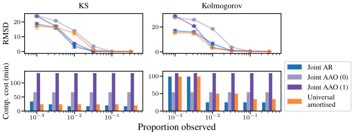
This figure displays the results of offline data assimilation experiments using four different methods: Joint AR, Joint AAO (0), Joint AAO (1), and Universal Amortised. The top row shows the Root Mean Squared Deviation (RMSD) for the Kuramoto-Sivashinsky (KS) and Kolmogorov flow datasets at various levels of data sparsity (proportion of observed data). The bottom row shows the computational cost (in minutes) for each method and sparsity level. The results indicate that the AR method generally outperforms the AAO methods, especially in sparse data scenarios, though using more corrector steps (AAO(1) vs AAO(0)) improves AAO accuracy. The Universal Amortised method shows competitive performance.

This figure shows three example trajectories generated by solving the Burgers’ equation. The trajectories represent the training, validation, and test sets. Each trajectory shows the evolution of the solution over time (from t=0s to t=1s), with the spatial dimension discretized into 128 points. The parameters used in generating these examples are consistent with the setup described in reference [77]. All three trajectories have the same length. The time-step used is ∆τ = 0.01s.

This figure shows examples of training, validation, and testing trajectories from the Kuramoto-Sivashinsky dataset. The key difference highlighted is the length of the trajectories: training trajectories are shorter (140 time steps, 0-28 seconds), while validation and testing trajectories are longer (640 time steps, 0-128 seconds). The spatial resolution is consistent across all examples (256 evenly distributed states).
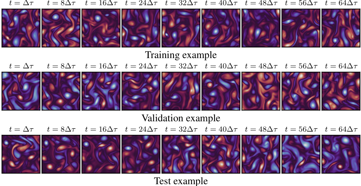
This figure shows examples of the Kolmogorov flow dataset used in the paper. The dataset consists of 2D PDE trajectories (velocity fields) at different time points. The figure displays 3 example trajectories from the training, validation, and test sets of the dataset. Each row shows a different trajectory. Within each row, different time steps (t) are shown in different frames. The visualization emphasizes the time evolution of the complex, swirling patterns characteristic of the Kolmogorov flow.

This figure compares the performance of two different solvers (DPM++ and EI) and two different time schedules (quadratic and linear) for generating samples using the all-at-once (AAO) approach. The results are shown for different numbers of corrector steps (0, 5, and 25). It shows that with few corrector steps, the choice of solver and time schedule does not affect the results significantly, but with 25 corrector steps, the quadratic time schedule performs slightly better.

This figure shows the impact of different solvers (DPM++, EI) and time scheduling methods (quadratic, linear) on the Root Mean Square Deviation (RMSD) for the Burgers’ equation. The left, middle and right panels show results for 0, 5, and 25 corrector steps respectively. The results indicate that with few corrector steps, solver and scheduling choices have little impact on the RMSD. However, with 25 corrector steps, the quadratic time schedule shows lower RMSD.

This figure displays box plots comparing the root mean squared error (RMSE) for different solver and time scheduling methods when applied to the Burgers’ equation. Three levels of corrector steps (0, 5, 25) are shown, for two solvers (DPM++, EI) and two time scheduling approaches (linear, quadratic). The results show relatively little difference in RMSE between the solvers and time scheduling methods when the number of corrector steps is low; however, with 25 corrector steps the quadratic schedule shows a noticeably lower RMSE.

The figure is a box plot showing the results of the RMSD for the Burgers’ dataset for different numbers of corrector steps using two different solvers (DPM++ and EI) and two different time schedules (quadratic and linear). The plot shows that when using 0 or a small number of corrector steps, the RMSD is not significantly affected by the choice of solver or time schedule. However, when using 25 corrector steps, the quadratic time schedule appears to produce slightly lower RMSD values.

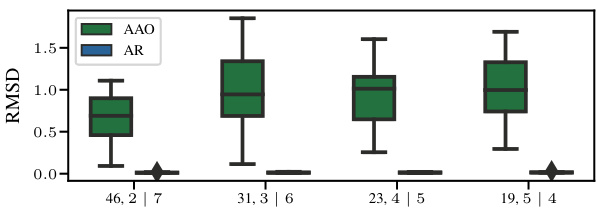
This figure compares the root mean square deviation (RMSD) between the generated samples and true trajectories for both All-at-once (AAO) and Autoregressive (AR) sampling methods on the Burgers’ dataset. The window size used for the score network was 5. The number of corrector steps for AAO was chosen to match the computational cost of AR sampling with 0 corrector steps. The results show that AR sampling, which iteratively generates states conditioned on previous ones, significantly outperforms the AAO approach, which generates the entire trajectory at once. This demonstrates the superior performance of the AR method for forecasting PDE dynamics.
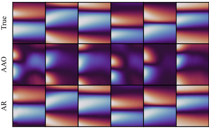
This figure compares the true samples, AAO samples, and AR samples for the Burgers’ dataset. The top row shows the ground truth. The middle row shows AAO samples, which only correctly capture the initial states. The bottom row shows the AR samples, which maintain a good correlation with the ground truth even for long trajectories of 101 timesteps. This demonstrates the superiority of AR sampling over AAO sampling for long-term prediction.
This figure compares the Root Mean Squared Deviation (RMSD) for the Burgers’ equation using two different solvers (DPM++ and EI) and two different time schedules (quadratic and linear). It shows results for 0, 5, and 25 corrector steps. The key takeaway is that with few corrector steps, the solver and schedule choice have minimal impact on the accuracy, but with many (25) steps, the quadratic schedule is slightly better.

This figure shows a comparison of true, predicted (using joint AR model), and interpolated trajectories against the observed data for Kolmogorov dataset. The top part shows the case where 10% of the data was observed while the bottom part shows the case where 1% of the data was observed. The predicted trajectory using the joint AR model generally more closely matches the observed data than the interpolated trajectory.

This figure compares the performance of All-at-once (AAO) and Autoregressive (AR) sampling methods on the Burgers’ dataset. The top panel shows the true values. The middle panel shows the AAO samples. The bottom panel shows the AR samples. The AAO method only captures the initial states correctly, while the AR method maintains a good correlation with the ground truth throughout the entire 101 time steps of the trajectory.
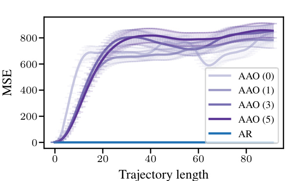
This figure displays the results of an experiment comparing the performance of two different solvers (DPM++ and EI) and two time scheduling methods (quadratic and linear) for the Burgers’ equation. The mean squared error (MSE) is calculated for varying numbers of corrector steps (0, 5, and 25). The results show that with few corrector steps, the choice of solver and scheduling method has little impact on the MSE. However, with 25 corrector steps, the quadratic time scheduling method shows a slight advantage in terms of lower RMSD.

This figure compares the Root Mean Squared Deviation (RMSD) for the Burgers’ equation using two different solvers (DPM++ and EI) and two different time schedules (quadratic and linear) for generating samples. The results are displayed for different numbers of corrector steps (0, 5, and 25). The key finding is that when using few or no corrector steps, the RMSD is relatively insensitive to the solver or time schedule. However, with many corrector steps (25), the quadratic time schedule shows a slightly lower RMSD.

This figure shows example trajectory snapshots from the Kolmogorov dataset. The training, validation, and test trajectories all have 64 time steps. Only a subset of these time steps (t ∈ {∆τ, 8∆τ, 16∆τ, 24∆τ, 32∆τ, 40∆τ, 48∆τ, 56∆τ, 64∆τ}) are displayed for each example to illustrate the flow and evolution of the dataset.

This figure compares the performance of three different diffusion models (Joint AR, Amortised, and Universal Amortised) on two different datasets (KS and Kolmogorov) for the task of forecasting. The x-axis represents different combinations of P (number of generated states) and C (number of conditioned states), representing varying lengths of forecasting and history lengths used. The y-axis represents the high correlation time which indicates the forecasting ability of the model. The longer the high correlation time the better the model is at accurately forecasting the future states. Error bars are included to show the uncertainty in measurements. The results indicate that the universal amortised model generally performs better.
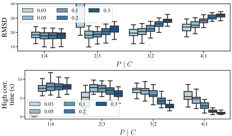
This figure shows the forecasting performance of the joint model on the Kolmogorov dataset. It explores the impact of different values of the guidance strength parameter (γ) and various conditioning scenarios (P|C) on both the root mean squared deviation (RMSD) and high correlation time. The top row displays the RMSD for different P|C settings and gamma values, while the bottom row shows the corresponding high correlation times. The results help illustrate how different parameter choices affect the model’s ability to forecast accurately and for how long.

This figure shows the root mean square deviation (RMSD) and computational cost for different data assimilation scenarios. The top row displays the RMSD error for the Kuramoto-Sivashinsky (KS) and Kolmogorov flow equations, comparing the performance of the models as the proportion of observed data varies from very sparse to fully observed. The bottom row illustrates the computational cost for each scenario, highlighting that the autoregressive (AR) approach’s cost is dependent on the specific conditioning parameters (P|C), unlike the all-at-once (AAO) approach.

This figure compares the forecasting performance of three different diffusion models (joint, amortised, and universal amortised) across various conditioning scenarios. The x-axis represents different combinations of generated states (P) and conditioned states (C), while the y-axis displays the high correlation time, a metric evaluating the accuracy and consistency of long-term predictions. Error bars represent the mean ± 3 standard errors calculated from test trajectories.

This figure compares the forecasting performance of three different diffusion models (Joint AR, Amortised, and Universal Amortised) on two datasets (KS and Kolmogorov). The x-axis shows different combinations of P (number of states generated) and C (number of states conditioned on) during sampling, which represents the model’s ability to extrapolate from a history of observations. The y-axis shows the high correlation time, which measures the accuracy and length of the forecast. The results show that the Universal Amortised model achieves the best performance in most scenarios, indicating superior ability to handle forecasting under various history lengths.

This figure displays the root mean square deviation (RMSD) and computation cost for different data sparsity levels in offline data assimilation for the Kuramoto-Sivashinsky (KS) and Kolmogorov flow equations. The top panels show RMSD, demonstrating how the error varies with the proportion of observed data. The bottom panels illustrate the computational cost. Autoregressive (AR) methods show better performance in sparse observation settings but increase computation time with the amount of data.

The figure compares the forecasting performance of the joint AR and universal amortised models against two common baselines: persistence and climatology. The mean squared error (MSE) is plotted against trajectory length for both the Kuramoto-Sivashinsky (KS) and Kolmogorov datasets. Error bars represent ± 3 standard errors. The results show that both models significantly outperform climatology for a substantial portion of the trajectory length, indicating their ability to capture the underlying dynamics better than simply predicting the average value or the previous value.
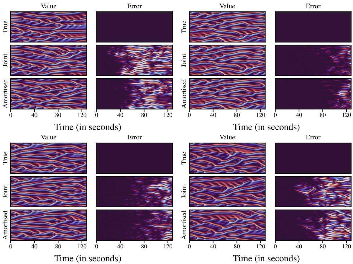
This figure compares the performance of the joint and universal amortised models on the Kuramoto-Sivashinsky (KS) dataset for forecasting. The top row shows the ground truth trajectories. The middle row shows the predictions from the joint model, which uses 1 state for prediction and 8 states for conditioning. The bottom row shows the predictions from the universal amortised model, which uses 8 states for prediction and 1 state for conditioning. The right-hand column shows the error between the predictions and ground truth for each model. The top-left example corresponds to a trajectory where both models perform well, and the top-right example corresponds to a trajectory where the models’ predictions are less accurate.

This figure compares the vorticity fields generated by the joint and universal amortised models with the ground truth for the Kolmogorov dataset. It shows results for four different initial conditions and at eight time points (t = Δτ, t = 9Δτ, t = 17Δτ, t = 25Δτ, t = 33Δτ, t = 41Δτ, t = 49Δτ, t = 57Δτ). Each row displays the results for one model (ground truth, joint, amortised), making it easy to visually assess the differences between models in generating realistic fluid flow patterns at various times.

This figure shows the results of the offline data assimilation experiment using the joint model with a window size of 9 on the Kuramoto-Sivashinsky (KS) dataset. It compares the performance of the all-at-once (AAO) sampling method with 0 and 1 corrector steps, across various levels of sparsity (indicated on the x-axis as the ‘proportion observed’). Different lines represent various values of γ, a hyperparameter controlling the guidance strength. The error bars represent ± 3 standard errors, indicating the uncertainty in the results.

The figure shows the results of the offline data assimilation experiments using the joint model and AAO sampling with 0 and 1 corrections. The x-axis represents the proportion of observed data, and the y-axis represents the RMSD. Different lines represent different values of the guidance strength (gamma). The results indicate that decreasing gamma (increasing guidance strength) too much can lead to decreased performance and larger standard errors.
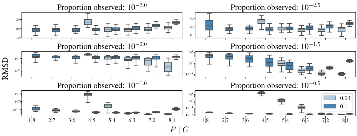
This figure compares the performance of different diffusion models on the offline data assimilation task. The top row of plots shows the root mean squared deviation (RMSD) for various sparsity levels (the proportion of observed data points), while the bottom row shows the computation time required for generating samples. The results demonstrate that the autoregressive (AR) approach is generally more efficient than the all-at-once (AAO) approach, especially for scenarios with sparse data. The performance difference between AR and AAO is particularly pronounced in cases with limited observations, highlighting the advantages of AR for data assimilation tasks.

This figure compares the performance of two different models for solving partial differential equations. The first model is a universal amortized model, which is a type of neural network that can be trained on many different data sets and then used to make predictions on new data sets. The second model is an amortized model, which is a type of neural network that is trained on a specific data set and then used to make predictions on new data sets of the same type. The figure shows that the universal amortized model is more stable and outperforms the amortized model across all combinations of parameters.

This figure compares the performance of two universal amortised models on the offline data assimilation task for the KS dataset. The left panel shows the root mean squared deviation (RMSD) for each model across various levels of observed data. One model uses only architectural conditioning, while the other uses reconstruction guidance to condition on sparse observations. The right panel visualizes the input data used by the models during each autoregressive (AR) step; this highlights how the model input changes as the sampling process progresses, revealing the difference in information available between models.

This figure compares the performance of two models with different window sizes (5 and 9) on the offline data assimilation task for the Kuramoto-Sivashinsky (KS) equation. The left panel shows results using autoregressive (AR) sampling, and the right panel displays results obtained using all-at-once (AAO) sampling with 0 and 1 correction. The x-axis represents the proportion of observed data, while the y-axis (RMSD) shows the root mean square deviation between the model prediction and the ground truth, illustrating the impact of window size and sampling method on data assimilation accuracy. Error bars show ± 3 standard errors.

This figure compares the performance of autoregressive (AR) sampling with all-at-once (AAO) sampling for offline data assimilation on the Kuramoto-Sivashinsky (KS) dataset. Two models are used: one with a window size of 5 and one with a window size of 9. The AAO model uses 0, 1, and 2 corrector steps. The results show that AR sampling generally outperforms AAO sampling, especially at lower proportions of observed data. The right-hand plot presents the data on a logarithmic scale to better visualize the differences between the methods across different sparsity levels.

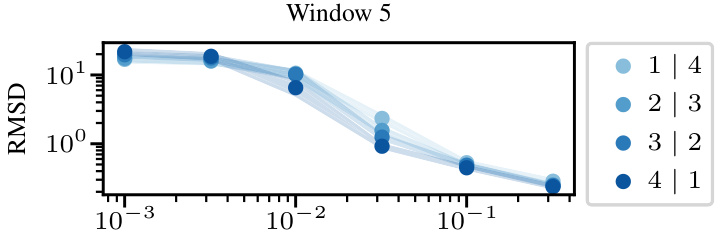
This figure compares the root mean squared deviation (RMSD) for different conditioning scenarios (P|C) in offline data assimilation using two different diffusion models. The x-axis shows the proportion of observed data, ranging from very sparse to nearly full observation. The y-axis represents the RMSD, measured on a logarithmic scale. The left panel corresponds to a model with a window of size 5, while the right panel represents a model with a window of size 9. Each line represents a different P|C conditioning scenario (where P is the number of states predicted per iteration and C is the number of conditioning states). The figure demonstrates the impact of the conditioning scenarios and the window size on the accuracy of the models.

This figure compares the Root Mean Squared Deviation (RMSD) and computational cost of different models for offline data assimilation (DA) tasks on the Kuramoto-Sivashinsky (KS) and Kolmogorov datasets. The top part of the figure shows the RMSD for various levels of data sparsity. The bottom part shows the computational cost (in minutes) associated with each model and sparsity level. The results demonstrate that autoregressive (AR) sampling achieves better performance, especially in low-data regimes, but at a higher computational cost compared to the all-at-once (AAO) approach which is quicker but less accurate.
This figure compares the forecasting performance of three different diffusion models (Joint AR, Amortised, and Universal Amortised) on two datasets (KS and Kolmogorov). The x-axis represents different conditioning scenarios, specified by the parameters P (number of generated states) and C (number of conditioned states). The y-axis shows the high correlation time, a measure of forecasting accuracy. Error bars represent the mean ± 3 standard errors, indicating the statistical significance of the results. The figure demonstrates the impact of different conditioning strategies on model performance across varying data complexities.

This figure compares the Root Mean Squared Deviation (RMSD) and computational cost of different models on the offline data assimilation (DA) task for the Kuramoto-Sivashinsky (KS) and Kolmogorov flow equations. The top row shows the RMSD for various sparsity levels (i.e., proportions of observed data). The bottom row shows the computational cost for each sparsity level and for different sampling methods (AAO and AR). The key observation is that AR generally outperforms AAO, especially in sparse data regimes, but that its computational cost is higher, with the difference in cost also varying with the number of correction steps used.

This figure compares the true trajectories of the Kuramoto-Sivashinsky (KS) equation with the predictions made by the joint autoregressive (AR) model and the results obtained using a simple interpolation method. It showcases the performance of the model under different levels of data sparsity (10% and 1%). The top row displays the original true trajectories and the corresponding observed, sparsely sampled data. The bottom row presents the model’s predictions alongside the results of the interpolation technique. This visualization is intended to highlight the model’s ability to capture the underlying dynamics even when a substantial portion of the data is missing, thereby contrasting its performance against a simpler interpolation approach.
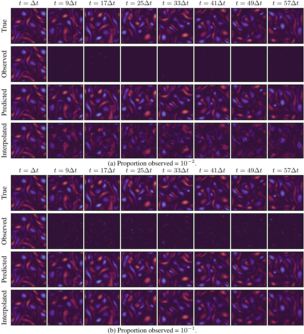
This figure compares the true, predicted (using the joint AR model), and interpolated trajectories of the Kuramoto-Sivashinsky (KS) equation, alongside the observed values, for two different proportions of observed data: 10⁻² (left) and 10⁻¹ (right). The comparison visually demonstrates the model’s ability to capture the underlying dynamics of the KS equation, especially when compared to simple interpolation, which struggles to accurately reconstruct the trajectory, particularly in sparser data conditions.

This figure illustrates the setup for the online data assimilation task using the Kuramoto-Sivashinsky (KS) dataset. The task involves forecasting future states while incorporating sparse observations that arrive every 20 time steps. At each step, the model uses a block of 20 sparse observations and its previous forecast to predict the next 400 states. This process continues until the entire trajectory of length 640 is predicted, demonstrating how the model handles both forecasting and data assimilation simultaneously.

This figure compares the performance of the joint model on the Kuramoto-Sivashinsky (KS) and Kolmogorov datasets in the online data assimilation task for varying conditioning scenarios. The x-axis represents different combinations of P (number of states generated at each iteration) and C (number of conditioned states). For KS, a window size of 9 is used; for Kolmogorov, the window size is 5. The RMSD (root mean squared error) is shown for each combination of P and C, indicating the model’s forecasting accuracy under different levels of data sparsity.

This figure compares the performance of different diffusion models on the offline data assimilation task. The top row shows the root mean squared deviation (RMSD) of the model predictions from the ground truth, for varying levels of data sparsity, indicating the amount of observed data. The models are Joint AR (autoregressive), Joint AAO (all-at-once), and Universal Amortised. The bottom row shows the computational cost of each approach. AAO has a consistent computational cost for all sparsity levels, whereas AR’s cost varies with the choice of the hyperparameter P|C. The results demonstrate that AR generally outperforms AAO for sparse data, but their performance is similar for dense data. The figure also highlights the impact of the number of corrector steps (c) in AAO on both accuracy and computational cost.

This figure compares the performance of three different diffusion models (joint, amortised, and universal amortised) on forecasting tasks for two different PDEs (Kuramoto-Sivashinsky and Kolmogorov). The performance is measured by the ‘high correlation time’, which reflects how long the model’s predictions accurately match the true trajectory. The x-axis shows different conditioning scenarios, where ‘P’ is the number of predicted states and ‘C’ is the number of conditioned states (i.e., states used as input to the model). The results show that the universal amortised model generally outperforms the other two models, especially for longer predictive horizons.

This figure compares the frequency spectrums of KS trajectories generated by different methods: Joint AR, universal amortised, PDE-Refiner, MSE-trained U-Net, and MSE-trained FNO. Each row shows the spectrum for a different trajectory, with the left column displaying the spectrum of states closer to the initial state, and the right column showing states further from the initial state. The analysis aims to show how well each method captures the high-frequency components of the trajectories, which is important for long-term forecasting accuracy.

This figure shows a comparison of long-term predictions for the Kuramoto-Sivashinsky equation using three different approaches: the ground truth, the joint AR model and the universal amortized model. The results demonstrate that both the joint AR and universal amortized models can generate reasonably realistic trajectories even for time periods much longer than those seen in training.

This figure compares the frequency spectra of different models’ predictions against the ground truth for a long trajectory. The top row shows results for states close to the beginning, the middle row for states in the middle, and the bottom row for states close to the end of the trajectory. The plot helps visualize how well different models (Joint AR and Universal Amortised) capture the frequency characteristics of the true data at different points in time along the trajectory.
More on tables

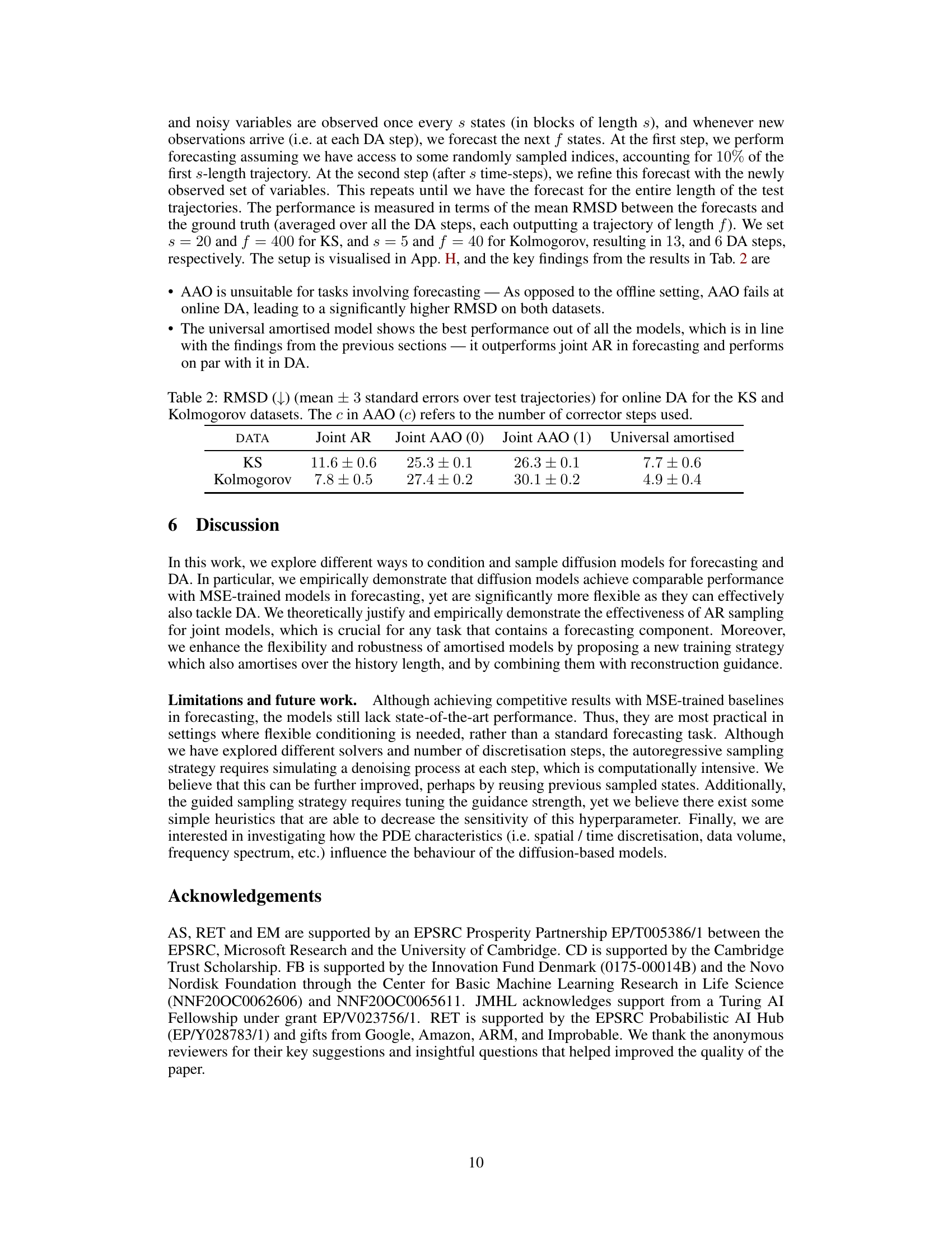
This table presents the results of the online data assimilation experiments. It shows the root mean squared deviation (RMSD) for the Kuramoto-Sivashinsky (KS) and Kolmogorov datasets. Different models are compared: Joint AR, Joint AAO (0), Joint AAO (1), and Universal Amortised. The number after the parentheses in ‘Joint AAO’ indicates the number of corrector steps used in the sampling process. Lower RMSD values indicate better performance.
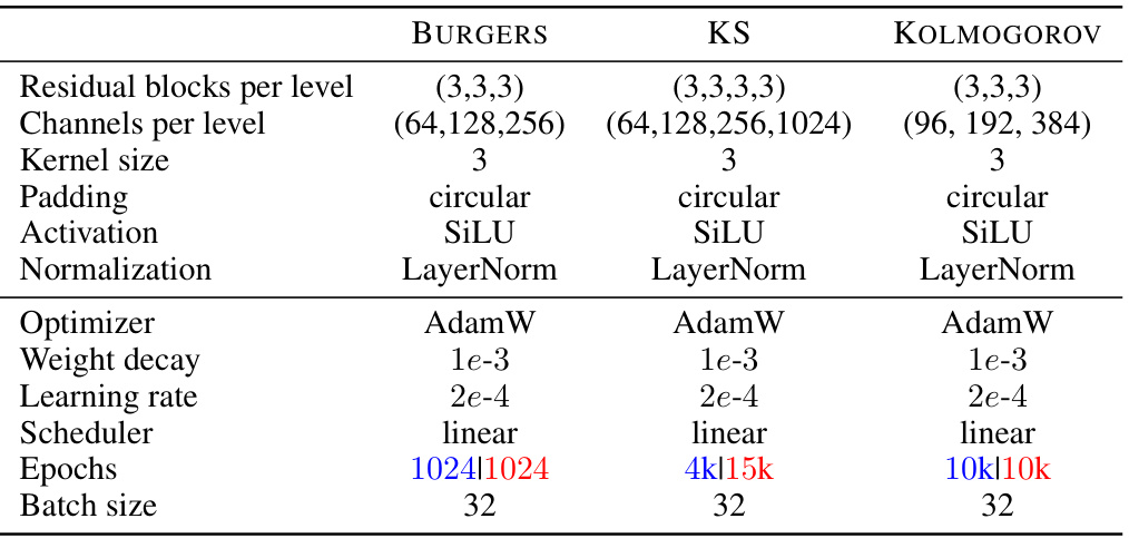
This table lists the hyperparameters used for training the score-based diffusion models. The hyperparameters are specific to each dataset (Burgers, KS, Kolmogorov) and model type (joint or universal amortised). The table shows choices made for the following: residual blocks per level, channels per level, kernel size, padding, activation function, normalization method, optimizer, weight decay, learning rate, scheduler, number of epochs, and batch size.

This table presents the hyperparameters used for training the PDE-Refiner U-Net architecture, inspired by the work of [42], in the forecasting experiments. It includes details about residual blocks per level, channels per level, kernel size, padding, activation, normalization, optimizer, weight decay, learning rate, scheduler, epochs and batch size for both Kuramoto-Sivashinsky (KS) and Kolmogorov datasets. The table highlights the specific differences in hyperparameters between the joint and universal amortised models using blue and red color coding.

This table presents the best high correlation time achieved by four different models (Joint AR, Univ. Amortised, Amortised, and MSE U-Net) using two different architectures (SDA and PDE-Refiner) across two datasets (KS and Kolmogorov). The best performance for each model/architecture combination, along with the corresponding conditioning parameters (P|C), is shown. The results highlight the variation in performance between different models and architectures across the two datasets.

This table shows the best value of the guidance strength hyperparameter (γ) for different conditioning scenarios (P) and varying proportions of observed data for the Kolmogorov dataset. The experiments were performed using a joint model with a window size of 5. The optimal value of γ appears to be dependent on both the conditioning scenario and the proportion of data observed.
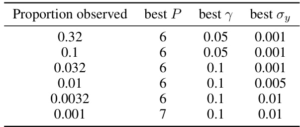
This table shows the best hyperparameter settings (γ, σy, P) for the universal amortised model with a window size of 9, for different proportions of observed data in the offline data assimilation task on the Kuramoto-Sivashinsky (KS) dataset. The parameters were tuned to optimize the model’s performance for each sparsity level. The best predictive horizon (P), guidance strength (γ), and observation noise standard deviation (σy) are presented for each data sparsity level.

This table shows the best hyperparameter settings for the universal amortised model on the Kolmogorov dataset for different levels of data sparsity. For each proportion of observed data, the table shows the best predictive horizon (P), guidance strength (γ), and observation noise standard deviation (σy). These settings were determined empirically through a hyperparameter sweep and aim to optimize performance in data assimilation tasks within the model.
Full paper#
