Estimating Generalization Performance Along the Trajectory of Proximal SGD in Robust Regression

↗ OpenReview ↗ NeurIPS Homepage ↗ Chat

TL;DR

#

Key Takeaways

#

Why does it matter?

#

This paper is crucial for researchers in robust regression and optimization. It directly addresses the challenge of accurately estimating generalization error during iterative model training, improving model selection and tuning. The proposed consistent estimators, applicable to various algorithms and loss functions, offer significant advantages for practical applications. Furthermore, it paves the way for new research into improving iterative algorithm analysis, particularly in high-dimensional settings.

Visual Insights

#

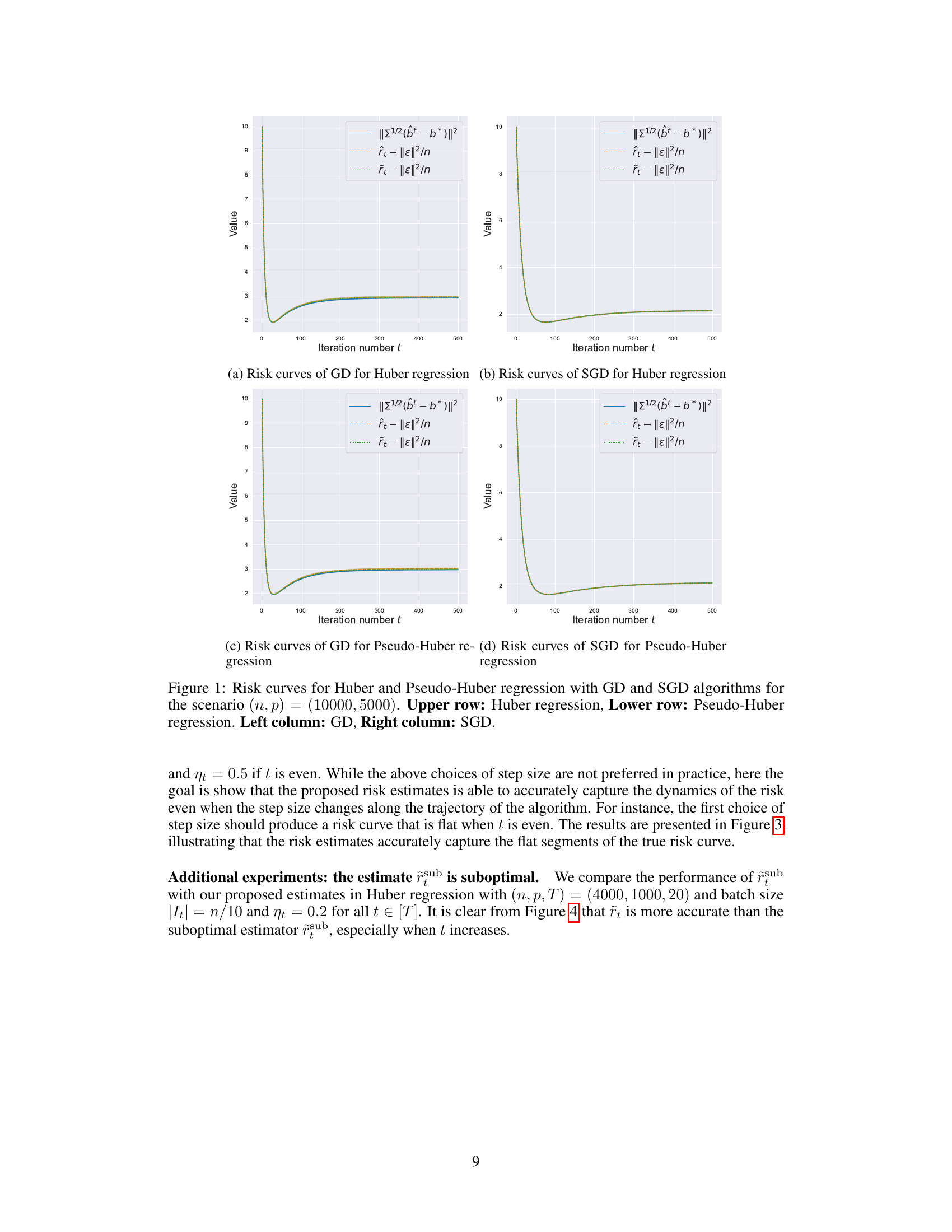
This figure displays the risk curves for Huber and Pseudo-Huber regression using Gradient Descent (GD) and Stochastic Gradient Descent (SGD) methods. The scenario uses a sample size (n) of 10000 and a feature dimension (p) of 5000. The top row shows results for Huber regression, while the bottom row shows results for Pseudo-Huber regression. The left column presents the results for the GD algorithm, and the right column for SGD. Each curve shows the actual risk (||∑^1/2(b̂_t - b*)||^2), and the two estimates (r̂_t - ||ε||^2/n and r̃_t - ||ε||^2/n) with their 2 standard error bars. The graph helps in visually comparing the performance of different algorithms and evaluating the accuracy of the proposed risk estimates.

This table summarizes the specifications of the functions ψ, φt, and matrices St used in the general iterative algorithm (4) for different algorithms: Gradient Descent (GD), Stochastic Gradient Descent (SGD), Proximal Gradient Descent, and Proximal Stochastic Gradient Descent. The functions ψ and φt represent the data fitting loss and update functions respectively, while St represents the diagonal matrix used for batch updates in SGD and Proximal SGD.

In-depth insights

#

Proximal SGD Track

#

A Proximal Stochastic Gradient Descent (SGD) track in a research paper would likely involve analyzing the algorithm’s behavior when dealing with non-smooth (non-differentiable) penalty functions in the optimization problem. Proximal methods are crucial here because they efficiently handle the non-smoothness, unlike standard gradient descent. The track could explore how the generalization performance of proximal SGD changes along the optimization trajectory. Key aspects could include the development of consistent generalization error estimators specific to proximal SGD, potentially adapting existing methods or devising novel ones. It might also investigate optimal stopping criteria – determining when to stop the algorithm to achieve the best generalization. The analysis would likely involve theoretical convergence guarantees, supported by empirical validation. Specific examples of non-smooth penalties (such as L1 regularization or other sparsity-inducing penalties) would be used to illustrate practical applications and performance differences compared to standard SGD. In essence, a comprehensive proximal SGD track aims to provide a thorough understanding of this variant’s capabilities and limitations in the context of the research problem.

Robust Risk Estimator

#

A robust risk estimator is crucial for reliable machine learning model evaluation, especially when dealing with high-dimensional data or heavy-tailed noise. Robustness implies the estimator is insensitive to outliers or violations of assumptions about data distribution. This is particularly important in real-world applications where data is often noisy and may not conform to idealized statistical models. A robust estimator would provide consistent and accurate risk estimates across a wide range of data characteristics, leading to more reliable model selection and hyperparameter tuning. Consistency ensures the estimator converges to the true risk as the sample size increases, while accuracy highlights its ability to provide precise risk estimations even with limited samples. The design of a robust risk estimator often involves techniques from robust statistics, such as using robust loss functions or regularization methods. Careful consideration of algorithmic bias and variance is vital for achieving both robustness and consistency.

High-Dim Robust Reg

#

High-dimensional robust regression (High-Dim Robust Reg) tackles the challenge of estimating regression coefficients when the number of predictors (p) is comparable to or exceeds the number of observations (n), and the data is contaminated with outliers or heavy-tailed noise. Traditional regression methods often fail in this setting because they are sensitive to outliers and can overfit the data, leading to poor generalization performance. Robust regression techniques aim to mitigate these issues by employing loss functions less sensitive to outliers (like Huber or Tukey loss), which downweight the influence of extreme data points. In high dimensions, regularization is often essential to control overfitting and improve estimation accuracy; this commonly involves penalization methods such as LASSO or elastic net. A key difficulty in high-dimensional robust regression is the computational cost of many robust optimization methods. The development of efficient algorithms for solving the associated optimization problems remains an active area of research. Furthermore, theoretical analysis of estimation consistency and risk bounds is important to understand the performance guarantees of high-dimensional robust regression methods.

Generalization Error

#

Generalization error quantifies a model’s ability to perform on unseen data, crucial for evaluating machine learning algorithms. High generalization error suggests overfitting, where the model memorizes training data instead of learning underlying patterns. Conversely, low generalization error indicates good generalization, implying the model can accurately predict outcomes for new inputs. Estimating generalization error is challenging, often requiring computationally expensive techniques like cross-validation. The paper focuses on developing efficient estimators for generalization error specifically tailored for robust regression problems during the iterative optimization process. It addresses the issue of estimating generalization error at various points throughout an iterative algorithm, not just at convergence, offering a more granular understanding of model performance during training. The proposed method allows determining the optimal stopping point that minimizes this error, balancing model complexity against predictive accuracy. This is significant as it can aid in avoiding overfitting and improving the generalization performance of robust regression models.

Future Research

#

Future research directions stemming from this work could explore several promising avenues. Extending the theoretical framework to handle non-smooth loss functions beyond the Huber and Pseudo-Huber losses used in the current study is crucial. This would broaden the applicability of the proposed risk estimation techniques to a wider range of robust regression problems. Investigating the impact of different stochastic gradient descent variants and their hyperparameter settings on the accuracy of the risk estimates is essential. The study could analyze the effects of varying batch sizes, learning rates, and other hyperparameters to ascertain the robustness and efficiency of the proposed approach under different optimization scenarios. Developing a more refined understanding of the theoretical limitations and assumptions underlying the risk estimation methodology is also vital. This includes examining the impact of non-isotropic covariance matrices, correlated features, and heavy-tailed noise distributions on the consistency and accuracy of the estimates. Finally, the practical implications should be explored. Evaluating the efficacy of the proposed technique in real-world applications could reveal its effectiveness in diverse domains and identify areas needing further enhancement. The insights gained would improve the model’s utility for practitioners seeking to optimize the generalization performance of robust regression algorithms.

More visual insights

#

More on figures

This figure displays the risk curves for Huber and Pseudo-Huber regression using Gradient Descent (GD) and Stochastic Gradient Descent (SGD) methods. The experiment was conducted with a sample size (n) of 10,000 and feature dimension (p) of 5,000. The top row shows results for Huber regression, while the bottom row shows results for Pseudo-Huber regression. The left column shows results for GD, and the right column shows results for SGD. For each combination of regression type and optimization algorithm, the figure plots the actual risk (||∑^1/2(b^t - b*)||²), along with two estimates of this risk: î^t - ||ε||²/n and ř^t - ||ε||²/n, as well as their corresponding 2-standard-error bars. This visualization allows for comparison of the performance of different algorithms and the accuracy of the risk estimation methods.

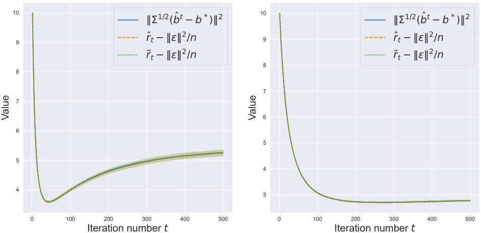
This figure displays the risk curves for Huber and Pseudo-Huber regression using Gradient Descent (GD) and Stochastic Gradient Descent (SGD) algorithms. The results are shown for two scenarios: (n, p) = (10000, 5000). Each plot shows the actual risk (||∑^1/2(b_t - b*)||²), along with two consistent estimates (î_t and r̃_t). The plots illustrate how the proposed estimates track the actual generalization error across different iterations of the algorithms and different regression types. The shaded region represents the 2 standard error bars.

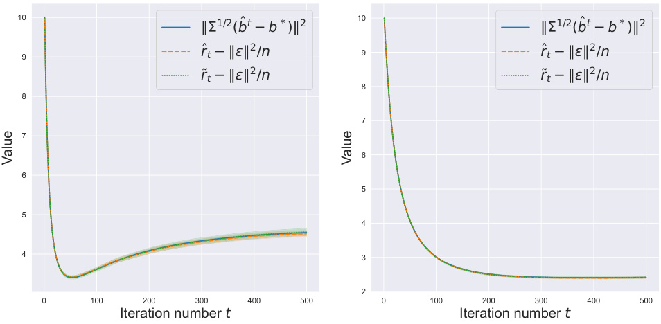
This figure displays the risk curves for Huber and Pseudo-Huber regression models using Gradient Descent (GD) and Stochastic Gradient Descent (SGD) algorithms. The simulations were run with a sample size of 10,000 and 5,000 features. The plots show the actual risk (||∑¹/²(b_t - b*)||²), and two proposed estimates (r̂_t - ||ε||²/n and r̃_t - ||ε||²/n) of the risk. The estimates closely track the actual risk, indicating their effectiveness in estimating generalization performance at different iterations of the algorithms.

This figure compares the performance of three risk estimators for SGD in Huber and pseudo-Huber regression. The estimators are: the actual risk, ||Σ^{1/2}(b_t - b^*)||^2, and two proposed estimators, \hat{r}_t - ||ε||^2/n and \tilde{r}_t - ||ε||^2/n. The plot shows the risk curves over 20 iterations. The figure demonstrates that the proposed estimators accurately track the true risk, even when using a constant step size.

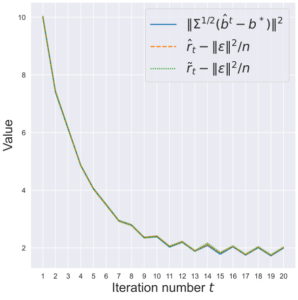
This figure compares the performance of the proposed risk estimators (î_t and r̃_t) with the true risk (||Σ^1/2(b̂_t - b*)||²) along the trajectory of Gradient Descent (GD) and Stochastic Gradient Descent (SGD) algorithms applied to both Huber and Pseudo-Huber regression problems. The top row shows the results for Huber regression, while the bottom row is for Pseudo-Huber regression. The left column presents results for the GD algorithm, and the right column presents those for the SGD algorithm. Each plot shows the true risk and the proposed estimators with error bars to illustrate the accuracy of the estimators.

This figure compares the performance of three risk estimators for SGD in Huber and pseudo-Huber regression. The estimators are: the actual risk ||Σ^1/2(b̂^t - b*)||², the proposed estimator r̂_t which is computationally efficient and does not require knowledge of Σ, the proposed estimator ˜r_t which requires knowledge of Σ, and the estimator r̃^sub_t obtained by directly generalizing the method from [5], which is suboptimal. The plot shows the risk curves for both Huber and pseudo-Huber regression along the iterations of the SGD algorithm. The results clearly indicate the superiority of the proposed estimators (r̂_t and ˜r_t) over the suboptimal method r̃^sub_t, demonstrating their effectiveness in accurately tracking the true risk.

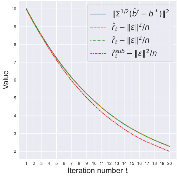
This figure compares the performance of three risk estimators: the proposed estimators r̂t and r̃t and the estimator r̂sub obtained by directly generalizing the approach in [5]. The plot shows that r̂t and r̃t more accurately estimate the true risk than r̂sub especially when the number of iterations increases.

Full paper

#