TL;DR#
Deep learning models often struggle with instability during training due to improper learning rate selection. A common practice to mitigate this is “learning rate warmup”, where the learning rate gradually increases from a small initial value to a target value. However, the reasons behind the success of warmup are not well understood. There are multiple hypotheses, but none provides a comprehensive explanation.
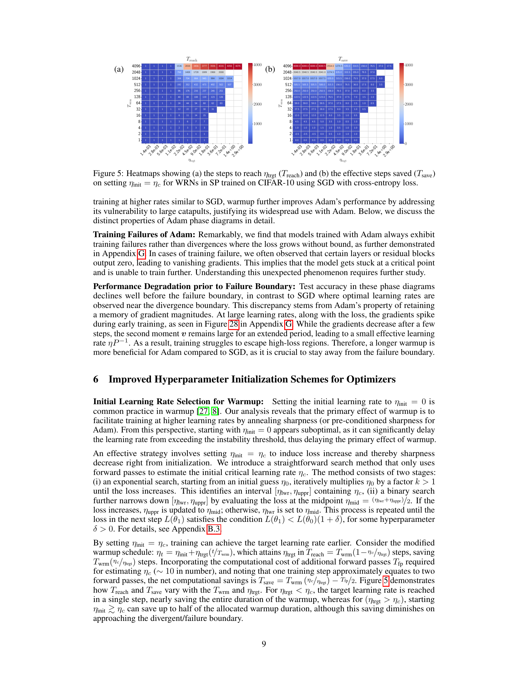
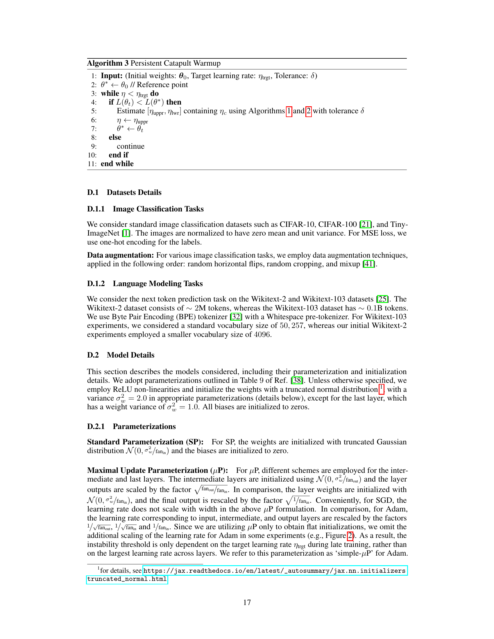
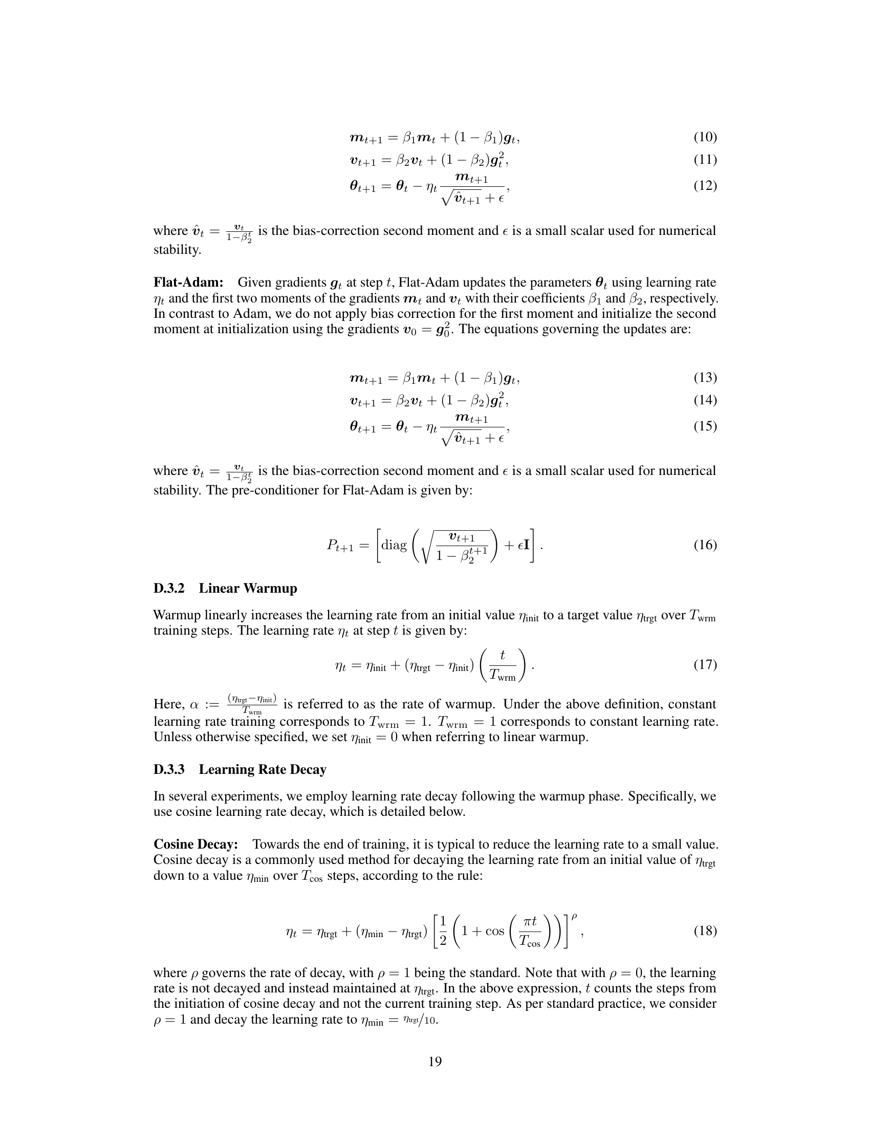
This paper uses systematic experiments to demonstrate that the primary benefit of warmup is its ability to allow the use of larger target learning rates. By carefully analyzing the sharpness of the loss landscape (or its preconditioned version for Adam), the authors identify different operational regimes during warmup. They also propose a modified Adam initialization, termed GI-Adam, that eliminates the need for warmup in some cases, and consistently improves performance.
Key Takeaways#
Why does it matter?#
This paper is crucial for researchers in deep learning optimization. It systematically investigates the often-used learning rate warmup technique, revealing its underlying mechanisms and suggesting improvements. This directly impacts the efficiency and robustness of training deep neural networks, which has broad implications for various applications.
Visual Insights#

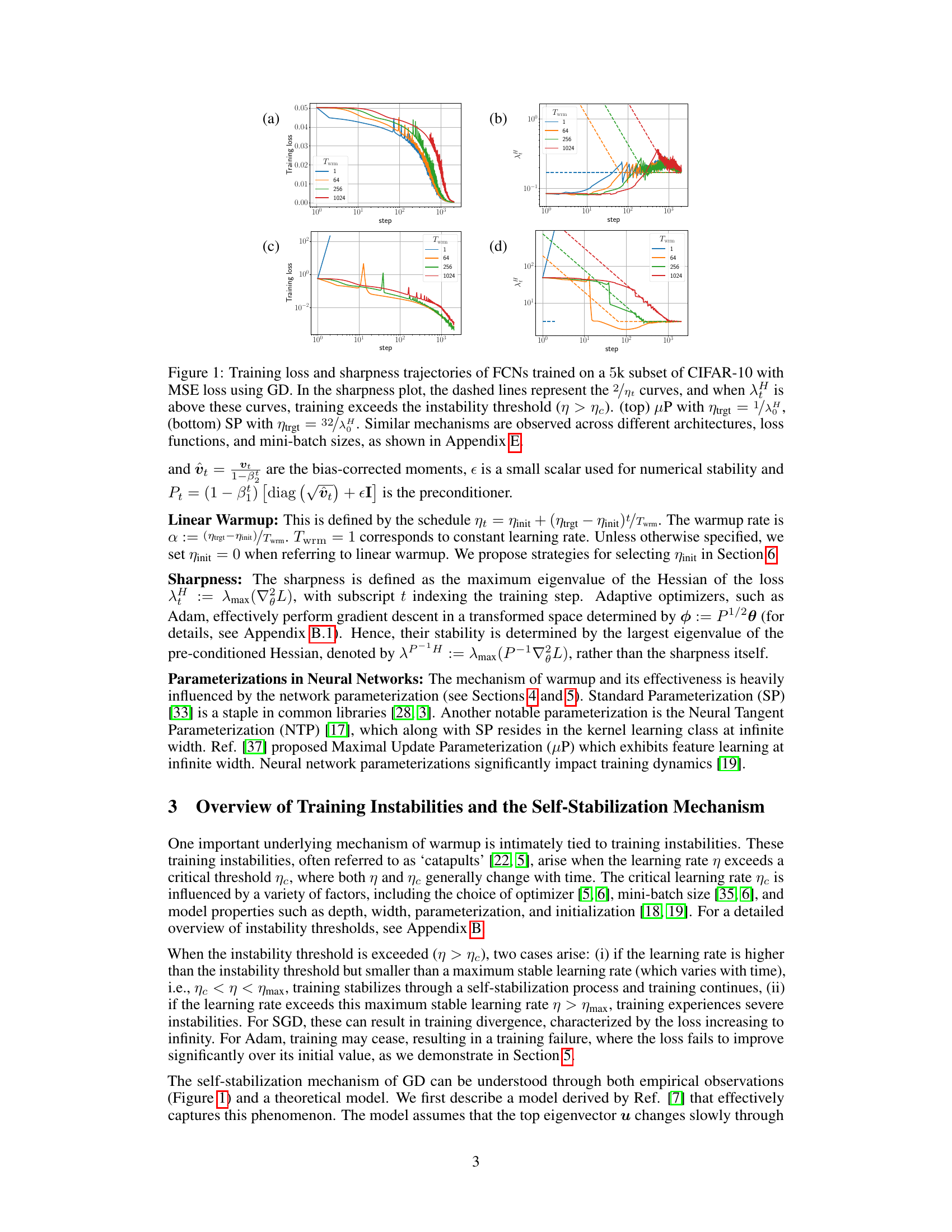
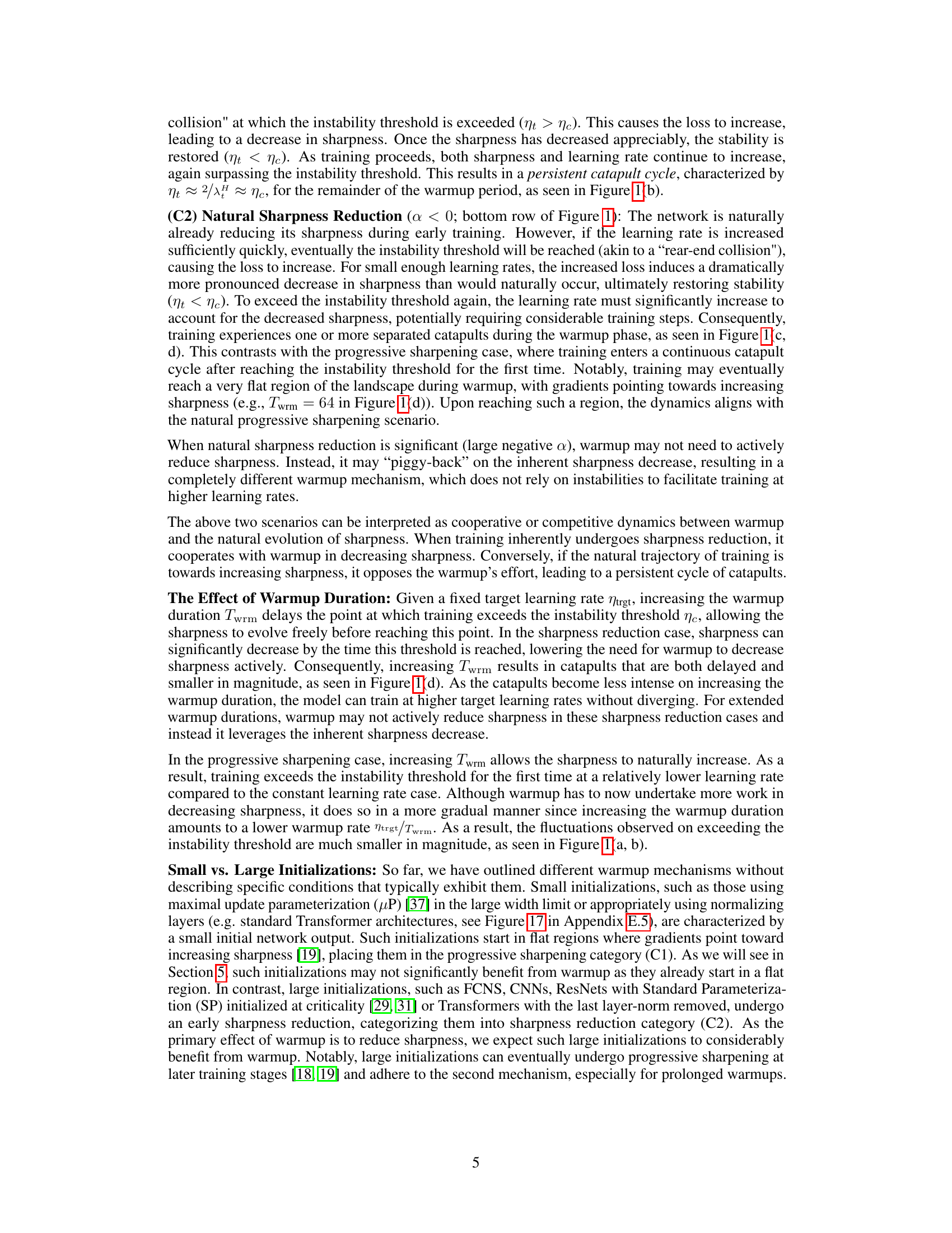
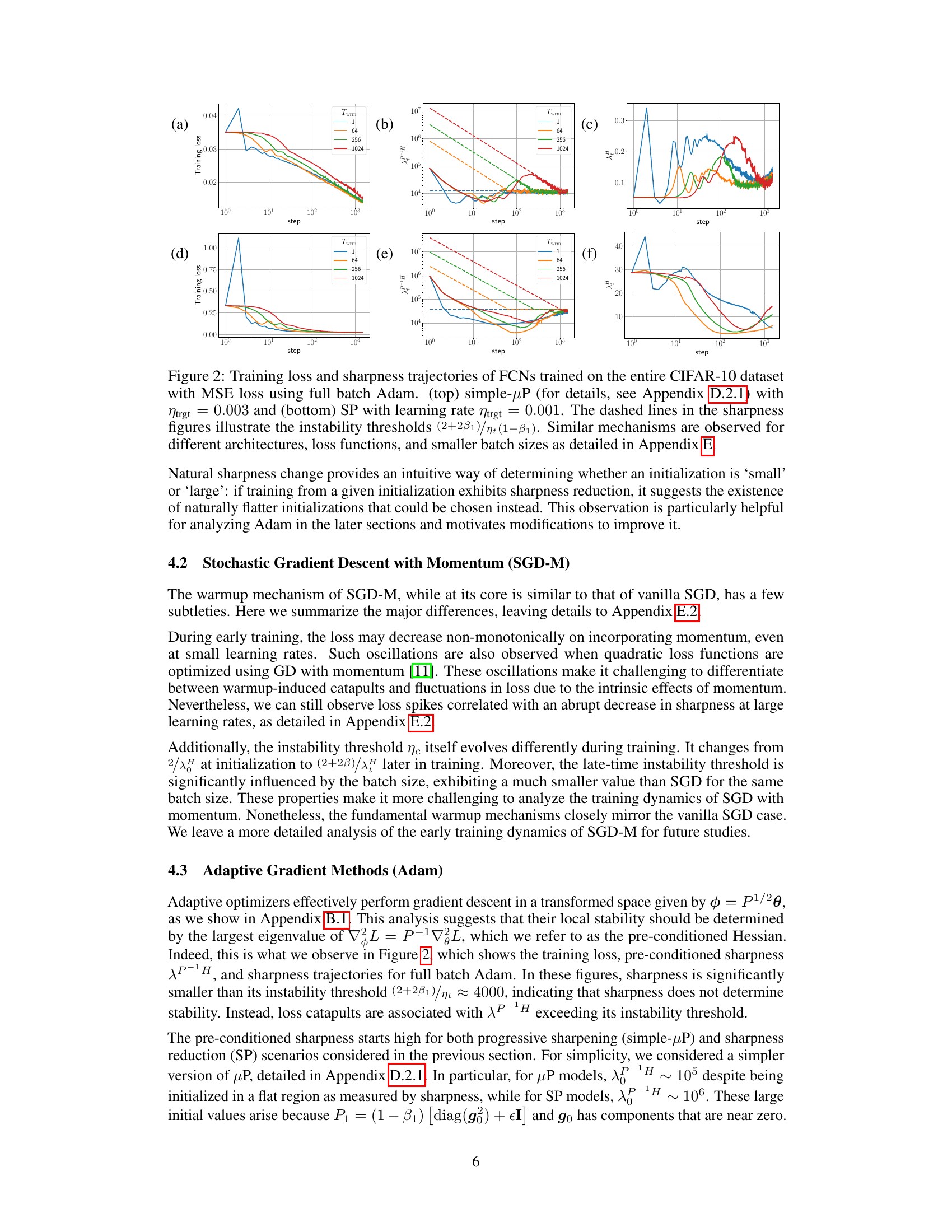
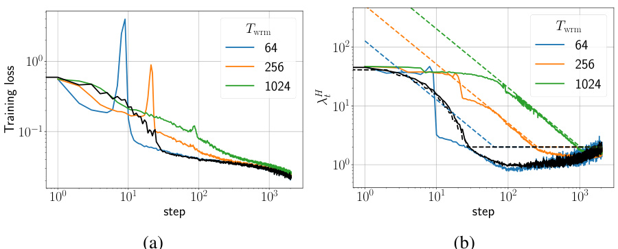
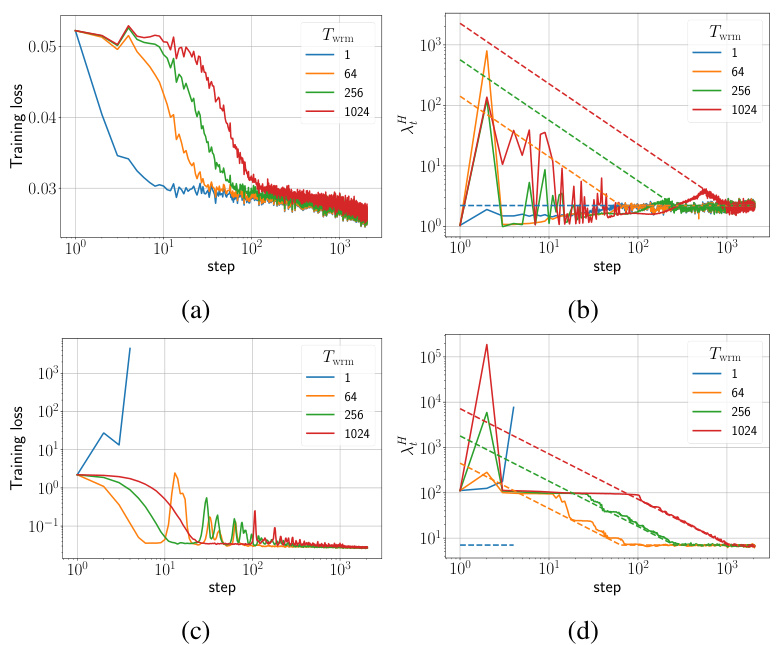
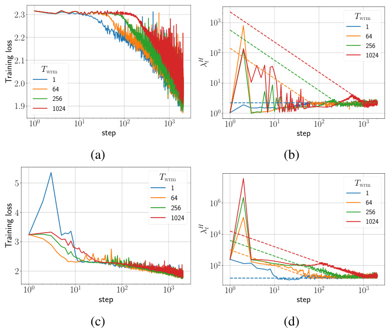
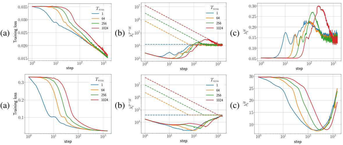
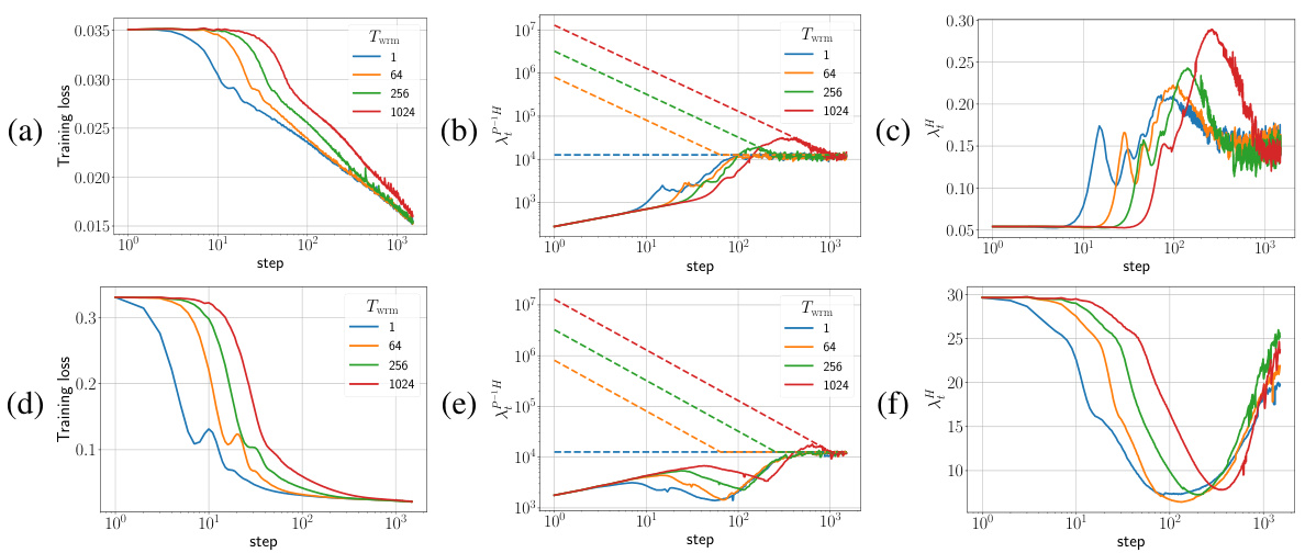
🔼 This figure shows the training loss and sharpness trajectories for two different parameterizations (μP and SP) of Fully Connected Networks (FCNs) trained on a subset of the CIFAR-10 dataset using gradient descent (GD) with a mean squared error (MSE) loss function. The sharpness is the maximum eigenvalue of the Hessian of the loss function. The dashed lines in the sharpness plots indicate the instability threshold (η > ηc), where η is the learning rate. When the sharpness exceeds this threshold, training becomes unstable. The top row shows the results for the μP parameterization, while the bottom row shows the results for the SP parameterization. Each parameterization uses a different target learning rate (ηtrgt). The figure illustrates how the learning rate warmup impacts the sharpness and loss curves during training, with the goal of preventing the network from entering unstable regions of the loss landscape.
read the caption
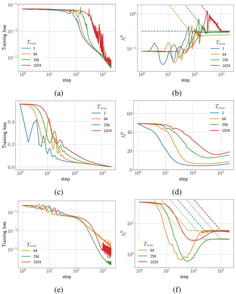
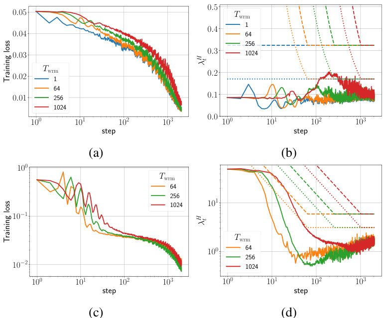
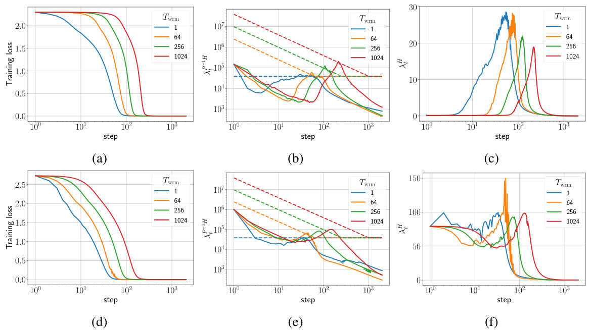
Figure 1: Training loss and sharpness trajectories of FCNs trained on a 5k subset of CIFAR-10 with MSE loss using GD. In the sharpness plot, the dashed lines represent the 2/ηt curves, and when λ is above these curves, training exceeds the instability threshold (η > ηc). (top) μP with ηtrgt = 1/8, (bottom) SP with ηtrgt = 32/λ. Similar mechanisms are observed across different architectures, loss functions, and mini-batch sizes, as shown in Appendix E.

🔼 This table compares the test accuracy achieved by different optimizers (Adam, GI-Adam, and RAdam) with varying warmup durations. The results show the mean and standard deviation of the test accuracy across multiple runs, highlighting the impact of warmup duration on the optimizer’s performance.
read the caption
Table 1: Performance comparison of different optimizers with varying warmup durations.
In-depth insights#
LR Warmup Benefits#
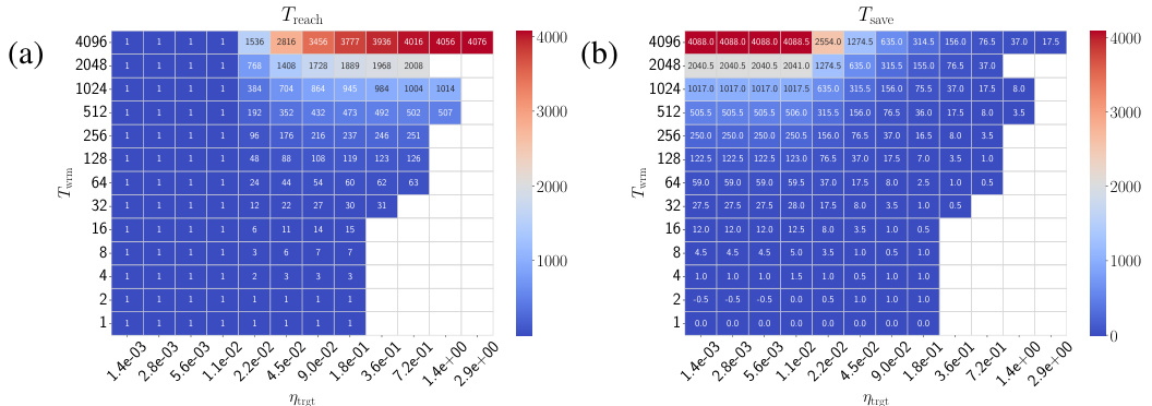
Learning rate warmup, a technique where the learning rate is gradually increased from a small initial value to a target value, offers several benefits in deep learning. Primarily, it enhances the robustness of training by allowing the network to tolerate larger target learning rates. This is crucial because larger learning rates can lead to faster convergence, potentially improving overall performance. However, excessively high learning rates can cause instability and divergence. Warmup acts as a buffer, easing the transition into this more aggressive training regime. It prevents large, destabilizing weight updates in the early stages of training, when the model is still highly sensitive to parameter changes. Further, warmup can help to reduce sharpness in the loss landscape, facilitating the model’s movement towards flatter regions conducive to effective optimization. This in turn enhances hyperparameter tuning robustness, as the network becomes less sensitive to the precise setting of the learning rate. Different initialization schemes and network architectures interact with warmup mechanisms in diverse ways, highlighting the importance of a deeper understanding to tailor the technique effectively for optimal outcomes. While increasing warmup duration can improve robustness, the main benefit typically stems from using a suitable target learning rate.
Sharpness Dynamics#
The concept of sharpness dynamics in the context of deep learning optimization is crucial. Sharpness, often represented as the maximum eigenvalue of the Hessian of the loss function, quantifies the curvature of the loss landscape around a model’s parameter values. High sharpness indicates a highly curved landscape, making optimization challenging because small changes in parameters lead to significant changes in the loss. Conversely, low sharpness indicates a flatter landscape, making optimization easier and more robust to larger learning rates. The paper explores how sharpness changes during training, specifically focusing on how different optimization techniques and hyperparameter settings impact this evolution. Warm-up strategies, for instance, aim to gradually reduce initial sharpness, allowing the network to learn effectively at higher learning rates later. The analysis of sharpness dynamics reveals different training regimes (progressive sharpening vs. sharpness reduction), which influences the effectiveness of strategies like warm-up. Understanding these dynamics provides critical insights for tuning hyperparameters and improving the robustness and efficiency of training deep learning models.
Adam Improvements#
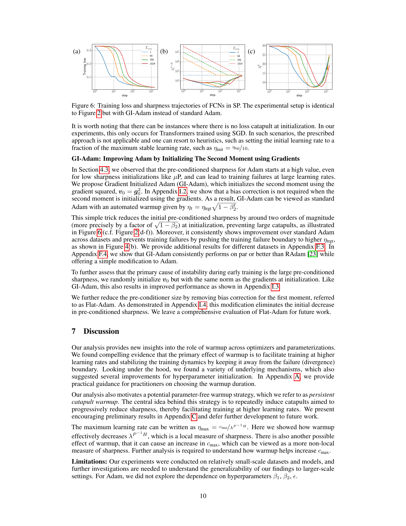
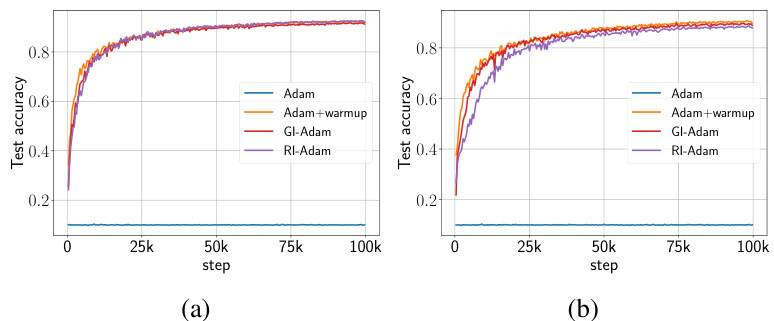
The research explores Adam optimizer improvements focusing on addressing training instabilities, particularly concerning the large pre-conditioned sharpness observed at initialization. A novel initialization strategy, GI-Adam, is proposed, which pre-initializes the second moment using gradients (v_0 = g_0). This simple modification significantly reduces the initial pre-conditioned sharpness, mitigating early instabilities that often lead to training failures. The study highlights that warmup’s primary benefit is to allow for larger target learning rates by gradually decreasing sharpness, thus enhancing the robustness of hyperparameter tuning and improving final performance. GI-Adam achieves similar benefits to warmup, sometimes eliminating the need for warmup entirely by pushing the training failure boundary to higher target learning rates. Furthermore, the analysis suggests that a more principled choice for the initial learning rate (η_init) can significantly reduce warmup time, sometimes making warmup unnecessary. The research provides compelling experimental evidence across various architectures, datasets, and optimizers, offering valuable insights and practical improvements to the Adam optimizer.
Warmup Regimes#
Analyzing “Warmup Regimes” in deep learning reveals distinct phases during the learning rate warmup period. These phases are not solely determined by the warmup schedule but are significantly influenced by the network’s initialization, architecture, and the loss landscape. Progressive sharpening, where sharpness increases over time, and sharpness reduction, where it decreases, represent two key regimes. The initial phase is crucial and dictates the subsequent behavior; whether a model begins in progressive sharpening or sharpness reduction will heavily influence how the learning rate increase affects the model’s stability and overall performance. Identifying this initial regime is key to optimizing the warmup process, allowing for tailored strategies to either leverage or mitigate its effects. Understanding these distinct regimes enables a more nuanced approach to warmup strategies, leading to improvements in training robustness and hyperparameter tuning.
Future Work#
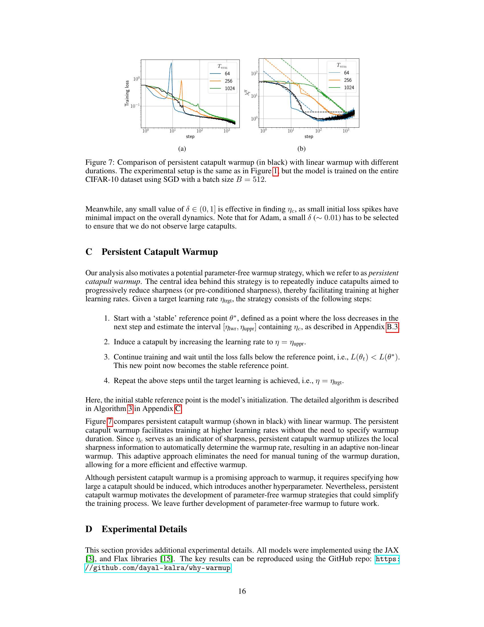
The paper’s lack of a dedicated ‘Future Work’ section presents an opportunity for insightful expansion. Investigating the self-stabilization mechanism in more complex optimizers beyond Adam is crucial. The current analysis primarily focuses on SGD and Adam; extending this to other adaptive methods or even different optimization families would significantly broaden the understanding of learning rate warmup’s impact. A deeper investigation into the interplay between the natural sharpness evolution and warmup’s impact, particularly for different model architectures and initializations, is warranted. This could lead to more sophisticated and tailored warmup strategies. Finally, the paper hints at a parameter-free warmup method using persistent catapults; fully developing and evaluating this approach could lead to more robust and efficient training across various tasks and settings. Further exploration into the use cases where warmup is not needed and identifying conditions for this would be beneficial.
More visual insights#
More on figures

🔼 This figure displays the training loss and sharpness trajectories of two different fully connected neural networks (FCNs) trained on a subset of the CIFAR-10 dataset using gradient descent (GD) with different initializations (μP and SP) and learning rate schedules. It shows how the learning rate affects the sharpness of the loss landscape and how training instability occurs when the learning rate exceeds a critical threshold. The top row shows results for the μP initialization, while the bottom row displays results for the SP initialization. The dashed lines in the sharpness plots indicate the threshold. Similar trends in network behavior are observed across various network architectures, loss functions, and batch sizes.
read the caption
Figure 1: Training loss and sharpness trajectories of FCNs trained on a 5k subset of CIFAR-10 with MSE loss using GD. In the sharpness plot, the dashed lines represent the λ/ηt curves, and when λ is above these curves, training exceeds the instability threshold (η > ηc). (top) μP with ηtrgt = 1/8, (bottom) SP with ηtrgt = 32/. Similar mechanisms are observed across different architectures, loss functions, and mini-batch sizes, as shown in Appendix E.
🔼 This figure shows the training loss and sharpness trajectories for two different parameterizations (μP and SP) of Fully Connected Networks (FCNs) trained on a subset of the CIFAR-10 dataset using gradient descent (GD). The top row displays results for the μP parameterization, and the bottom row shows results for the SP parameterization. The plots illustrate the relationship between the learning rate, sharpness, and training stability. The dashed lines in the sharpness plots represent instability thresholds; when the sharpness exceeds these thresholds, training becomes unstable. The figure shows different regimes of sharpness evolution during the warmup period that depend on initialization and parameterization.
read the caption
Figure 1: Training loss and sharpness trajectories of FCNs trained on a 5k subset of CIFAR-10 with MSE loss using GD. In the sharpness plot, the dashed lines represent the 2/ηt curves, and when λ is above these curves, training exceeds the instability threshold (η > ηc). (top) μP with ηtrgt = 1/8, (bottom) SP with ηtrgt = 32/. Similar mechanisms are observed across different architectures, loss functions, and mini-batch sizes, as shown in Appendix E.

🔼 This figure displays the training loss and sharpness trajectories for two different parameterizations (µP and SP) of Fully Connected Networks (FCNs) trained on a small subset of the CIFAR-10 dataset using Gradient Descent (GD). The plots show how the training loss and sharpness evolve over training steps for various warmup durations. The dashed lines in the sharpness plots represent thresholds above which training becomes unstable (η > ηc). The top row shows µP parameterization with a target learning rate (ηtrgt) set at 1/8, while the bottom row displays the SP parameterization with ηtrgt set to 32/λ, where λ is the sharpness. The results suggest that similar mechanisms are at play across different network architectures and training settings. Further details can be found in Appendix E.
read the caption
Figure 1: Training loss and sharpness trajectories of FCNs trained on a 5k subset of CIFAR-10 with MSE loss using GD. In the sharpness plot, the dashed lines represent the 2/ηt curves, and when λ is above these curves, training exceeds the instability threshold (η > ηc). (top) μP with ηtrgt = 1/8, (bottom) SP with ηtrgt = 32/λ. Similar mechanisms are observed across different architectures, loss functions, and mini-batch sizes, as shown in Appendix E.
🔼 This figure shows the training loss and sharpness trajectories for two different parameterizations (μP and SP) of Fully Connected Networks (FCNs) trained on a subset of the CIFAR-10 dataset using gradient descent (GD) with different warmup durations. The sharpness plots illustrate the relationship between sharpness, learning rate, and training stability, showing when training surpasses a critical threshold. The results highlight the impact of parameterization and learning rate schedules on training stability and the effectiveness of warmup in mitigating instabilities.
read the caption
Figure 1: Training loss and sharpness trajectories of FCNs trained on a 5k subset of CIFAR-10 with MSE loss using GD. In the sharpness plot, the dashed lines represent the 2/nt curves, and when λ is above these curves, training exceeds the instability threshold (η > ηc). (top) μP with ηtrgt = 1/8, (bottom) SP with ηtrgt = 32/. Similar mechanisms are observed across different architectures, loss functions, and mini-batch sizes, as shown in Appendix E.

🔼 This figure displays the training loss and sharpness trajectories for two different parameterizations (μP and SP) of Fully Connected Networks (FCNs) trained on a subset of the CIFAR-10 dataset using gradient descent (GD). The sharpness plots show the maximum eigenvalue of the Hessian of the loss function. Dashed lines indicate the instability threshold (η > ηc), where η is the learning rate. The figure illustrates how different parameterizations and learning rate warmup strategies impact the network’s stability and training dynamics.
read the caption
Figure 1: Training loss and sharpness trajectories of FCNs trained on a 5k subset of CIFAR-10 with MSE loss using GD. In the sharpness plot, the dashed lines represent the 2/ηt curves, and when λ is above these curves, training exceeds the instability threshold (η > ηc). (top) μP with ηtrgt = 1/8, (bottom) SP with ηtrgt = 32/. Similar mechanisms are observed across different architectures, loss functions, and mini-batch sizes, as shown in Appendix E.
🔼 This figure displays the training loss and sharpness trajectories for two different parameterizations (µP and SP) of Fully Connected Networks (FCNs) trained on a subset of the CIFAR-10 dataset using gradient descent (GD) with mean squared error (MSE) loss. The top row shows the µP parameterization, while the bottom row shows the SP parameterization. The plots illustrate the relationship between learning rate, training loss, and sharpness (the maximum eigenvalue of the Hessian of the loss). The dashed lines indicate the instability threshold (η > ηc), where the learning rate (η) is too high, causing training instabilities. The figure highlights how different parameterizations and learning rate schedules affect training dynamics and stability.
read the caption
Figure 1: Training loss and sharpness trajectories of FCNs trained on a 5k subset of CIFAR-10 with MSE loss using GD. In the sharpness plot, the dashed lines represent the 2/ηt curves, and when λ is above these curves, training exceeds the instability threshold (η > ηc). (top) μP with ηtrgt = 1/8, (bottom) SP with ηtrgt = 32/. Similar mechanisms are observed across different architectures, loss functions, and mini-batch sizes, as shown in Appendix E.

🔼 This figure shows the training loss and sharpness trajectories for two different parameterizations (µP and SP) of Fully Connected Networks (FCNs) trained on a subset of CIFAR-10 using Gradient Descent (GD) with different warmup durations. The sharpness is defined as the maximum eigenvalue of the Hessian of the loss function. The dashed lines in the sharpness plots indicate the instability thresholds (η > ηc). The figure demonstrates that warmup allows for training with larger target learning rates by facilitating a reduction in sharpness and moving the model away from unfavorable regions of the loss landscape. Similar trends are observed for different architectures and minibatch sizes.
read the caption
Figure 1: Training loss and sharpness trajectories of FCNs trained on a 5k subset of CIFAR-10 with MSE loss using GD. In the sharpness plot, the dashed lines represent the 2/ηt curves, and when λ is above these curves, training exceeds the instability threshold (η > ηc). (top) μP with ηtrgt = 1/8, (bottom) SP with ηtrgt = 32/. Similar mechanisms are observed across different architectures, loss functions, and mini-batch sizes, as shown in Appendix E.
🔼 This figure shows the training loss and sharpness trajectories for two different parameterizations (μP and SP) of Fully Connected Networks (FCNs) trained on a subset of CIFAR-10 dataset using Gradient Descent (GD) with different warmup durations. It demonstrates the relationship between learning rate, sharpness, and training stability, highlighting how warmup helps networks tolerate higher learning rates by forcing them into better-conditioned areas of the loss landscape. The dashed lines in the sharpness plots represent the instability threshold (2/η). When sharpness exceeds this threshold, training becomes unstable.
read the caption
Figure 1: Training loss and sharpness trajectories of FCNs trained on a 5k subset of CIFAR-10 with MSE loss using GD. In the sharpness plot, the dashed lines represent the 2/nt curves, and when λ is above these curves, training exceeds the instability threshold (η > ηc). (top) μP with ηtrgt = 1/8, (bottom) SP with ηtrgt = 32/. Similar mechanisms are observed across different architectures, loss functions, and mini-batch sizes, as shown in Appendix E.
🔼 This figure shows the training loss and sharpness trajectories for two different parameterizations (μP and SP) of a fully connected neural network (FCN) trained on a subset of the CIFAR-10 dataset using gradient descent (GD) with a mean squared error (MSE) loss function. The sharpness is plotted, showing the maximum eigenvalue of the Hessian matrix of the loss function. Dashed lines indicate the instability threshold (η > ηc), where η is the learning rate. The plots demonstrate how different parameterizations lead to variations in training dynamics and sharpness evolution, highlighting the concept of self-stabilization in training.
read the caption
Figure 1: Training loss and sharpness trajectories of FCNs trained on a 5k subset of CIFAR-10 with MSE loss using GD. In the sharpness plot, the dashed lines represent the λ/ηt curves, and when λ is above these curves, training exceeds the instability threshold (η > ηc). (top) μP with ηtrgt = 1/8, (bottom) SP with ηtrgt = 32/λ. Similar mechanisms are observed across different architectures, loss functions, and mini-batch sizes, as shown in Appendix E.

🔼 This figure shows the training loss and sharpness trajectories for two different parameterizations (μP and SP) of a Fully Connected Network (FCN) trained on a subset of the CIFAR-10 dataset using gradient descent (GD). The sharpness, representing the maximum eigenvalue of the Hessian of the loss function, is plotted against the training step. Dashed lines indicate instability thresholds. The figure demonstrates how warmup influences the network’s ability to tolerate higher target learning rates by affecting the sharpness. Different initializations and training phases (sharpness increase or decrease) lead to diverse training dynamics.
read the caption
Figure 1: Training loss and sharpness trajectories of FCNs trained on a 5k subset of CIFAR-10 with MSE loss using GD. In the sharpness plot, the dashed lines represent the 2/ηt curves, and when λ is above these curves, training exceeds the instability threshold (η > ηc). (top) μP with ηtrgt = 1/8, (bottom) SP with ηtrgt = 32/λ. Similar mechanisms are observed across different architectures, loss functions, and mini-batch sizes, as shown in Appendix E.

🔼 The figure shows the training loss and sharpness trajectories of two fully connected networks (FCNs) trained on a subset of the CIFAR-10 dataset using gradient descent (GD) with different warmup durations. The top row shows the results for a network with maximal update parameterization (μP), and the bottom row shows the results for a network with standard parameterization (SP). The dashed lines in the sharpness plots indicate the instability threshold. The figure illustrates how different warmup schedules affect the ability of the network to handle larger learning rates and demonstrates the self-stabilization mechanism.
read the caption
Figure 1: Training loss and sharpness trajectories of FCNs trained on a 5k subset of CIFAR-10 with MSE loss using GD. In the sharpness plot, the dashed lines represent the 2/nt curves, and when λ is above these curves, training exceeds the instability threshold (η > ηc). (top) μP with ηtrgt = 1/8, (bottom) SP with ηtrgt = 32/. Similar mechanisms are observed across different architectures, loss functions, and mini-batch sizes, as shown in Appendix E.

🔼 This figure shows the training loss and sharpness trajectories for two different parameterizations (µP and SP) of Fully Connected Networks (FCNs) trained on a subset of CIFAR-10 dataset using Gradient Descent (GD) with different warmup durations. The top row shows the results for the µP parameterization, while the bottom row shows the results for the SP parameterization. The plots illustrate how the learning rate warmup affects the training stability and sharpness of the model, with longer warmup periods leading to greater stability and potentially better final performance. The dashed lines in the sharpness plots represent the theoretical instability threshold.
read the caption
Figure 1: Training loss and sharpness trajectories of FCNs trained on a 5k subset of CIFAR-10 with MSE loss using GD. In the sharpness plot, the dashed lines represent the 2/ηt curves, and when λ is above these curves, training exceeds the instability threshold (η > ηc). (top) μP with ηtrgt = 1/8, (bottom) SP with ηtrgt = 32/. Similar mechanisms are observed across different architectures, loss functions, and mini-batch sizes, as shown in Appendix E.
🔼 This figure shows the training loss and sharpness trajectories for two different network parameterizations (μP and SP) trained on a subset of CIFAR-10 using gradient descent (GD) with varying warmup durations. The top row shows the results for the μP parameterization, while the bottom row shows the results for the SP parameterization. The dashed lines in the sharpness plots represent the instability thresholds. When the sharpness is above these thresholds, training becomes unstable. This instability is mitigated by using a warmup period, which allows the network to gradually adjust to the larger learning rate.
read the caption
Figure 1: Training loss and sharpness trajectories of FCNs trained on a 5k subset of CIFAR-10 with MSE loss using GD. In the sharpness plot, the dashed lines represent the 2/nt curves, and when λ is above these curves, training exceeds the instability threshold (η > ηc). (top) μP with ηtrgt = 1/8, (bottom) SP with ηtrgt = 32/. Similar mechanisms are observed across different architectures, loss functions, and mini-batch sizes, as shown in Appendix E.
🔼 This figure displays the training loss and sharpness trajectories for two different parameterizations (μP and SP) of a Fully Connected Network (FCN) trained on a subset of the CIFAR-10 dataset using gradient descent (GD). The top row shows the results for the μP parameterization, while the bottom row shows the results for the SP parameterization. Sharpness is plotted against the training step. Dashed lines indicate the instability thresholds, illustrating the relationship between learning rate, sharpness and stability during training. Different warmup durations are shown, and the figure demonstrates the self-stabilization mechanism where training approaches, exceeds, and then recovers from an instability threshold.
read the caption
Figure 1: Training loss and sharpness trajectories of FCNs trained on a 5k subset of CIFAR-10 with MSE loss using GD. In the sharpness plot, the dashed lines represent the λ/ηt curves, and when λ is above these curves, training exceeds the instability threshold (η > ηc). (top) μP with ηtrgt = 1/8, (bottom) SP with ηtrgt = 32/λ. Similar mechanisms are observed across different architectures, loss functions, and mini-batch sizes, as shown in Appendix E.
🔼 This figure shows the training loss and sharpness trajectories for two different parameterizations (μP and SP) of fully connected networks (FCNs) trained on a subset of the CIFAR-10 dataset using gradient descent (GD) with different warmup durations. The sharpness plots illustrate a critical learning rate (ηc) above which training becomes unstable. The top row demonstrates the µP parameterization, and the bottom row shows the SP parameterization. The key takeaway is the relationship between the learning rate, sharpness, and training stability, underscoring the influence of warmup on managing these dynamics.
read the caption
Figure 1: Training loss and sharpness trajectories of FCNs trained on a 5k subset of CIFAR-10 with MSE loss using GD. In the sharpness plot, the dashed lines represent the 2/ηt curves, and when λ is above these curves, training exceeds the instability threshold (η > ηc). (top) μP with ηtrgt = 1/8, (bottom) SP with ηtrgt = 32/λ. Similar mechanisms are observed across different architectures, loss functions, and mini-batch sizes, as shown in Appendix E.

🔼 This figure shows training loss and sharpness trajectories for fully connected networks (FCNs) trained on a subset of CIFAR-10 dataset. It compares two different parameterizations (μP and SP) with different warmup durations (Twrm). The dashed lines in the sharpness plots represent the instability threshold (ηc). The plots illustrate the self-stabilization mechanism where the training initially becomes unstable (η > ηc), then sharpness reduces, leading to stabilization.
read the caption
Figure 1: Training loss and sharpness trajectories of FCNs trained on a 5k subset of CIFAR-10 with MSE loss using GD. In the sharpness plot, the dashed lines represent the 2/ηt curves, and when λ is above these curves, training exceeds the instability threshold (η > ηc). (top) μP with ηtrgt = 1/8, (bottom) SP with ηtrgt = 32/λ. Similar mechanisms are observed across different architectures, loss functions, and mini-batch sizes, as shown in Appendix E.

🔼 This figure displays training loss and sharpness trajectories for two different parameterizations (µP and SP) of fully connected networks (FCNs) trained on a subset of the CIFAR-10 dataset using gradient descent (GD). The top row shows the µP parameterization, while the bottom row shows the SP parameterization. The plots illustrate how the learning rate warmup affects the training process by influencing the sharpness of the loss landscape. Dashed lines in the sharpness plots indicate the instability threshold, showing when the learning rate is too high for stable training. Different warmup durations (Twrm) are compared, illustrating how longer warmups allow the network to handle larger target learning rates.
read the caption
Figure 1: Training loss and sharpness trajectories of FCNs trained on a 5k subset of CIFAR-10 with MSE loss using GD. In the sharpness plot, the dashed lines represent the 2/ηt curves, and when λ is above these curves, training exceeds the instability threshold (η > ηc). (top) μP with ηtrgt = 1/8, (bottom) SP with ηtrgt = 32/λ. Similar mechanisms are observed across different architectures, loss functions, and mini-batch sizes, as shown in Appendix E.
🔼 This figure shows the training loss and sharpness trajectories for two different parameterizations (μP and SP) of a fully connected network (FCN) trained on a small subset of the CIFAR-10 dataset using gradient descent (GD) with a mean squared error (MSE) loss function. The sharpness is the maximum eigenvalue of the Hessian of the loss. The plots illustrate how the learning rate warmup affects the sharpness and the loss. The dashed lines represent the instability threshold, and when the sharpness exceeds this threshold, the training becomes unstable. The different initializations (μP and SP) affect the relationship between the learning rate and sharpness. The figure shows similar results across different architectures, mini-batch sizes, and loss functions, as detailed in Appendix E.
read the caption
Figure 1: Training loss and sharpness trajectories of FCNs trained on a 5k subset of CIFAR-10 with MSE loss using GD. In the sharpness plot, the dashed lines represent the 2/ηt curves, and when λ is above these curves, training exceeds the instability threshold (η > ηc). (top) μP with ηtrgt = 1/8, (bottom) SP with ηtrgt = 32/. Similar mechanisms are observed across different architectures, loss functions, and mini-batch sizes, as shown in Appendix E.
🔼 This figure shows the training loss and sharpness trajectories for two different parameterizations (µP and SP) of fully connected networks (FCNs) trained on a subset of the CIFAR-10 dataset using gradient descent (GD) with mean squared error (MSE) loss. The top row displays the results for the µP parameterization, and the bottom row shows the results for the SP parameterization. The dashed lines in the sharpness plots indicate the instability threshold (η > ηc), where η is the learning rate and ηc is the critical learning rate. The figure demonstrates how different network parameterizations impact the training dynamics and how the warmup period affects the ability of the network to reach and maintain stability at higher learning rates. It highlights the relationship between learning rate, loss, sharpness, and training stability.
read the caption
Figure 1: Training loss and sharpness trajectories of FCNs trained on a 5k subset of CIFAR-10 with MSE loss using GD. In the sharpness plot, the dashed lines represent the 2/ηt curves, and when λ is above these curves, training exceeds the instability threshold (η > ηc). (top) μP with ηtrgt = 1/8, (bottom) SP with ηtrgt = 32/λ. Similar mechanisms are observed across different architectures, loss functions, and mini-batch sizes, as shown in Appendix E.

🔼 This figure shows the training loss and sharpness trajectories for two different parameterizations (μP and SP) of a fully connected network (FCN) trained on a subset of the CIFAR-10 dataset using gradient descent (GD). The plots illustrate how the learning rate warmup affects training stability and sharpness. The dashed lines represent the instability thresholds, showing when the learning rate is too high for stable training. The top row demonstrates the μP parameterization, where the target learning rate is 1/8, while the bottom row illustrates the SP parameterization with a target learning rate of 32/. Similar behaviors are observed across different network architectures, loss functions, and batch sizes.
read the caption
Figure 1: Training loss and sharpness trajectories of FCNs trained on a 5k subset of CIFAR-10 with MSE loss using GD. In the sharpness plot, the dashed lines represent the 2/nt curves, and when λ is above these curves, training exceeds the instability threshold (η > ηc). (top) μP with ηtrgt = 1/8, (bottom) SP with ηtrgt = 32/. Similar mechanisms are observed across different architectures, loss functions, and mini-batch sizes, as shown in Appendix E.
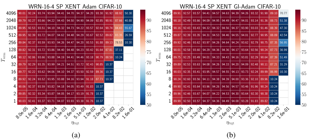
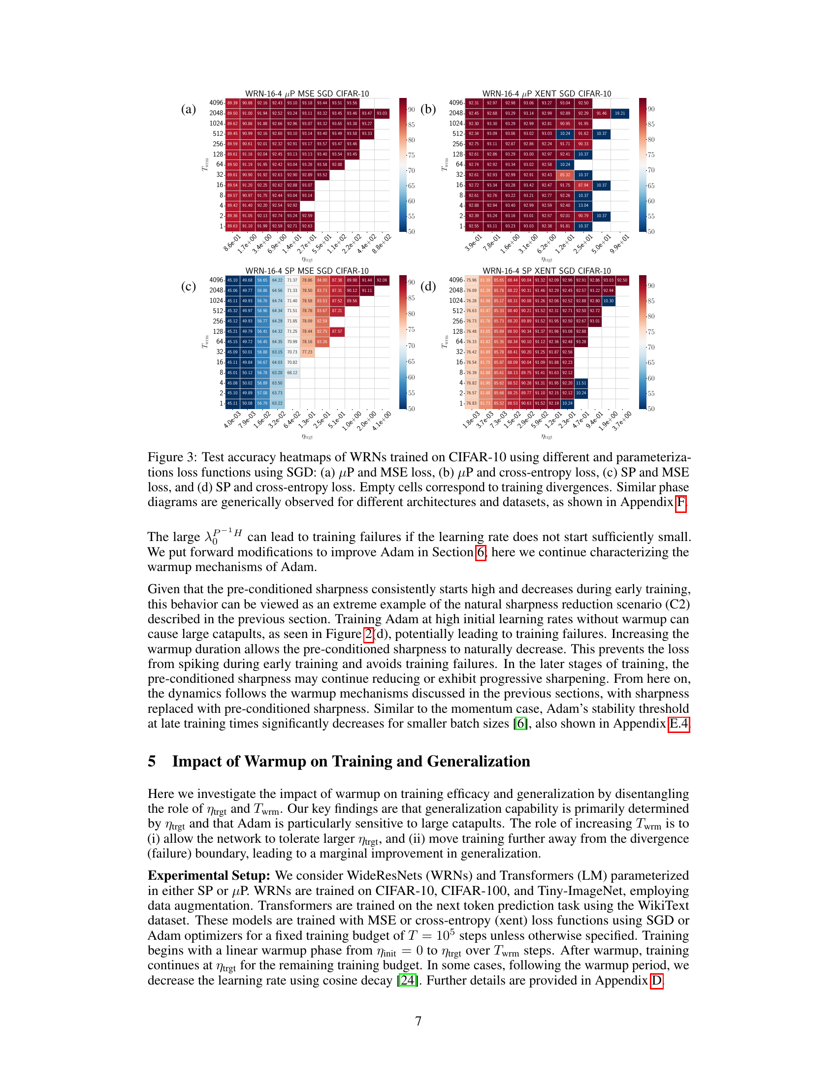
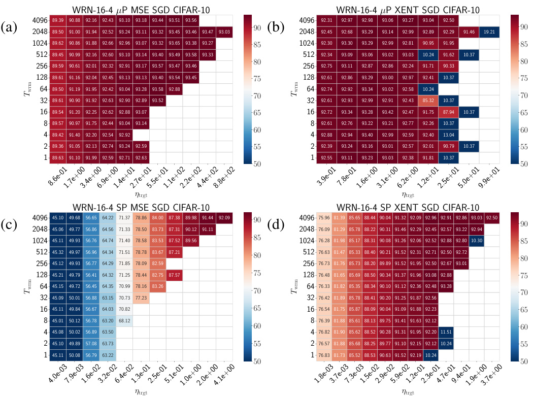
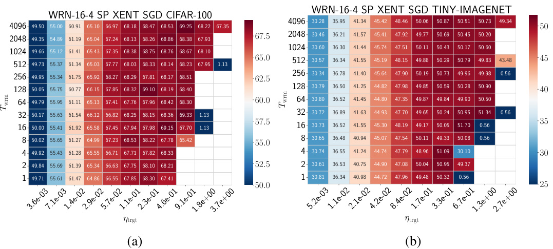
🔼 This figure shows the test accuracy for different combinations of network parameterization (μP or SP), loss function (MSE or cross-entropy), and warmup duration (Twrm) for Wide Residual Networks (WRNs) trained on CIFAR-10 using Stochastic Gradient Descent (SGD). Empty cells indicate that training diverged. The heatmaps demonstrate how the optimal hyperparameter settings are influenced by the interaction of parameterization, loss function, and warmup duration. Similar trends are observed across other architectures and datasets (see Appendix F for details).
read the caption
Figure 3: Test accuracy heatmaps of WRNs trained on CIFAR-10 using different parameterizations and loss functions using SGD: (a) μP and MSE loss, (b) μP and cross-entropy loss, (c) SP and MSE loss, and (d) SP and cross-entropy loss. Empty cells correspond to training divergences. Similar phase diagrams are generically observed for different architectures and datasets, as shown in Appendix F.
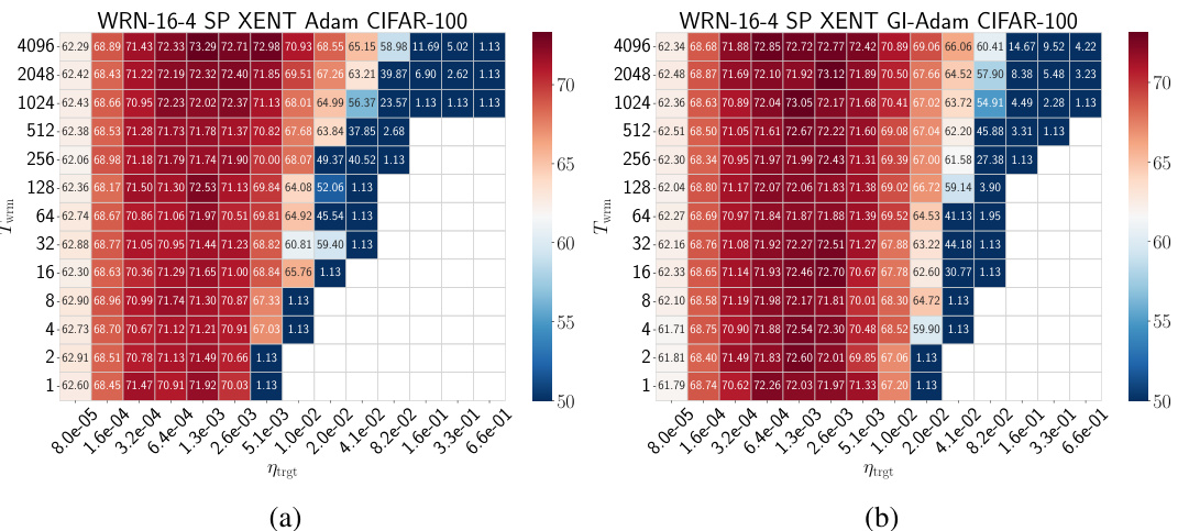
🔼 The figure shows heatmaps illustrating the test accuracy results for WideResNet (WRN) models trained on the CIFAR-10 dataset using different parameterizations (µP and SP) and loss functions (MSE and cross-entropy). The heatmaps depict how the test accuracy varies with respect to both the warmup duration (Twrm) and the target learning rate (ηtrgt). Empty cells indicate that training diverged for those parameter settings. The results show a similar pattern across different architectures and datasets, as detailed in Appendix F. The primary benefit of warmup is the ability to use larger learning rates.
read the caption
Figure 3: Test accuracy heatmaps of WRNs trained on CIFAR-10 using different parameterizations and loss functions using SGD: (a) µP and MSE loss, (b) µP and cross-entropy loss, (c) SP and MSE loss, and (d) SP and cross-entropy loss. Empty cells correspond to training divergences. Similar phase diagrams are generically observed for different architectures and datasets, as shown in Appendix F.

🔼 This figure shows the test accuracy results for WideResNet (WRN) models trained on the CIFAR-10 dataset using different parameterizations (μP and SP) and loss functions (MSE and cross-entropy). The heatmaps illustrate how the test accuracy varies with different target learning rates (ηtrgt) and warmup durations (Twrm). Empty cells indicate training divergences. The results demonstrate that the effect of warmup is robust across various architectural choices and loss functions, extending beyond the specific settings explored in the main body of the paper.
read the caption
Figure 3: Test accuracy heatmaps of WRNs trained on CIFAR-10 using different parameterizations and loss functions using SGD: (a) μP and MSE loss, (b) μP and cross-entropy loss, (c) SP and MSE loss, and (d) SP and cross-entropy loss. Empty cells correspond to training divergences. Similar phase diagrams are generically observed for different architectures and datasets, as shown in Appendix F.

🔼 This figure shows the training loss and sharpness trajectories for two different parameterizations (μP and SP) of Fully Connected Networks (FCNs) trained on a subset of the CIFAR-10 dataset using gradient descent (GD). The top row displays results for the μP parameterization, and the bottom row displays results for the SP parameterization. Different learning rates (η) are tested and the sharpness λ is plotted against the training steps. The dashed lines represent the stability threshold (ηc = 2/λ), where exceeding this threshold indicates instability. The figure illustrates how the choice of parameterization and the learning rate affects training stability and the relationship between loss and sharpness.
read the caption
Figure 1: Training loss and sharpness trajectories of FCNs trained on a 5k subset of CIFAR-10 with MSE loss using GD. In the sharpness plot, the dashed lines represent the 2/nt curves, and when λ is above these curves, training exceeds the instability threshold (η > ηc). (top) μP with ηtrgt = 1/8, (bottom) SP with ηtrgt = 32/. Similar mechanisms are observed across different architectures, loss functions, and mini-batch sizes, as shown in Appendix E.

🔼 This figure displays the training loss and sharpness trajectories for two different parameterizations (μP and SP) of a Fully Connected Network (FCN) trained on a subset of the CIFAR-10 dataset using Gradient Descent (GD) with a Mean Squared Error (MSE) loss function. The sharpness metric indicates the maximum eigenvalue of the Hessian of the loss. The dashed lines represent the instability threshold (ηc). The plots showcase how the learning rate warmup affects the training dynamics and stability for different network initializations.
read the caption
Figure 1: Training loss and sharpness trajectories of FCNs trained on a 5k subset of CIFAR-10 with MSE loss using GD. In the sharpness plot, the dashed lines represent the 2/ηt curves, and when λ is above these curves, training exceeds the instability threshold (η > ηc). (top) μP with ηtrgt = 1/8, (bottom) SP with ηtrgt = 32/. Similar mechanisms are observed across different architectures, loss functions, and mini-batch sizes, as shown in Appendix E.

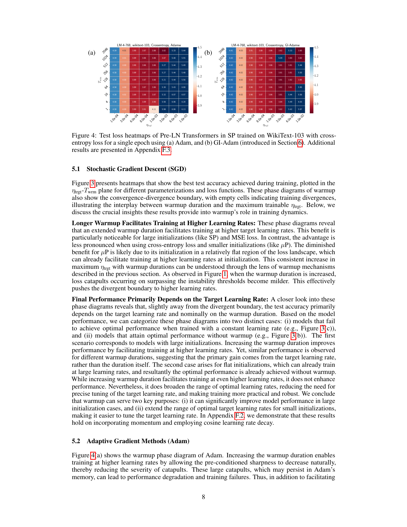
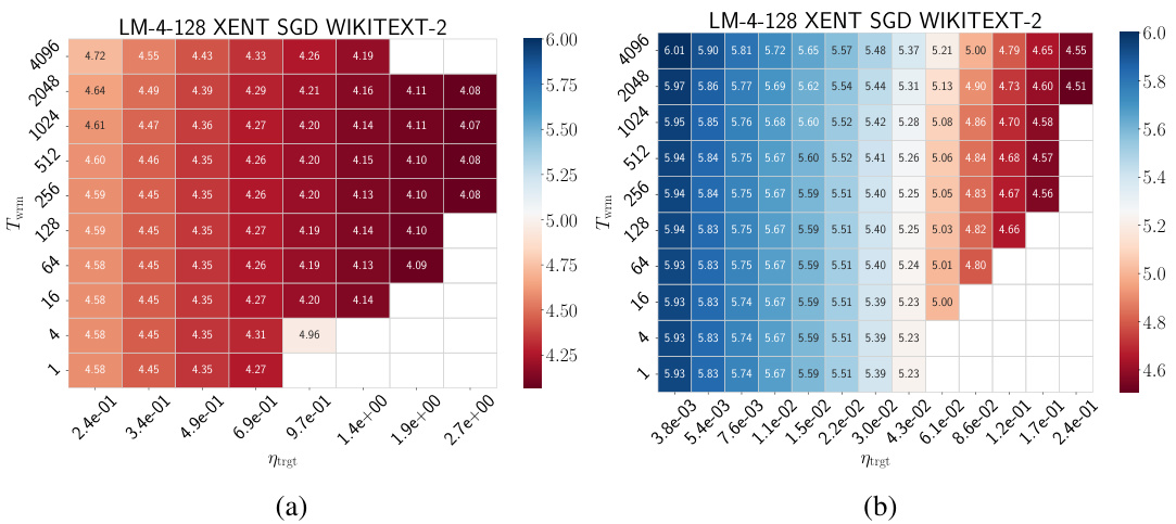
🔼 This figure displays heatmaps showing test loss of Pre-LN Transformers trained on the WikiText-103 dataset using Adam and GI-Adam optimizers. Each heatmap presents test loss as a function of the target learning rate (ηtrgt) and warmup duration (Twrm). The plots illustrate the performance differences between the standard Adam and the improved GI-Adam, particularly highlighting how GI-Adam allows for training with higher learning rates and reduces training failures. Appendix F.3 provides additional results.
read the caption
Figure 4: Test loss heatmaps of Pre-LN Transformers in SP trained on WikiText-103 with cross-entropy loss for a single epoch using (a) Adam, and (b) GI-Adam (introduced in Section 6). Additional results are presented in Appendix F.3.

🔼 This figure displays the training loss and sharpness trajectories for two different parameterizations (µP and SP) of fully connected networks (FCNs) trained on a subset of the CIFAR-10 dataset using gradient descent (GD) with a mean squared error (MSE) loss function. The sharpness is represented by the maximum eigenvalue of the Hessian. The dashed lines in the sharpness plots indicate instability thresholds. The top row shows the µP parameterization, while the bottom shows the SP parameterization. Each plot shows how the loss and sharpness change over training steps, illustrating how learning rate warmup affects training stability and sharpness. Similar behavior is observed in different architectures and loss functions.
read the caption
Figure 1: Training loss and sharpness trajectories of FCNs trained on a 5k subset of CIFAR-10 with MSE loss using GD. In the sharpness plot, the dashed lines represent the 2/nt curves, and when λ is above these curves, training exceeds the instability threshold (η > ηc). (top) μP with Ntrgt = 1/8, (bottom) SP with Ntrgt = 32/. Similar mechanisms are observed across different architectures, loss functions, and mini-batch sizes, as shown in Appendix E.
🔼 This figure shows training loss and sharpness trajectories for two different parameterizations (µP and SP) of fully connected networks (FCNs) trained on a subset of the CIFAR-10 dataset using gradient descent (GD). The sharpness plots illustrate how sharpness relates to the learning rate, and how a warmup schedule allows for higher target learning rates by avoiding instability.
read the caption
Figure 1: Training loss and sharpness trajectories of FCNs trained on a 5k subset of CIFAR-10 with MSE loss using GD. In the sharpness plot, the dashed lines represent the 2/nt curves, and when λ is above these curves, training exceeds the instability threshold (η > ηc). (top) μP with Ntrgt = 1/8, (bottom) SP with Ntrgt = 32/. Similar mechanisms are observed across different architectures, loss functions, and mini-batch sizes, as shown in Appendix E.
🔼 This figure displays the training loss and sharpness trajectories for two different parameterizations (μP and SP) of fully connected networks (FCNs) trained on a subset of the CIFAR-10 dataset. The plots illustrate how the learning rate warmup affects training stability. The dashed lines represent the instability threshold; when sharpness exceeds this threshold, training becomes unstable. The different warmup durations (Twrm) are compared, showing how they influence the sharpness and loss curves. The figure suggests that μP and SP exhibit different behaviors during the warmup period, which may relate to the sharpness reduction or sharpening phenomena discussed in the paper.
read the caption
Figure 1: Training loss and sharpness trajectories of FCNs trained on a 5k subset of CIFAR-10 with MSE loss using GD. In the sharpness plot, the dashed lines represent the 2/ηt curves, and when λ is above these curves, training exceeds the instability threshold (η > ηc). (top) μP with ηtrgt = 1/8, (bottom) SP with ηtrgt = 32/λ. Similar mechanisms are observed across different architectures, loss functions, and mini-batch sizes, as shown in Appendix E.

🔼 This figure displays the training loss and sharpness trajectories of two different types of fully connected neural networks (FCNs) trained on a subset of the CIFAR-10 dataset using gradient descent (GD) with different learning rates. The top row shows the results for a network initialized using the maximal update parameterization (µP), while the bottom row shows the results for a network initialized using the standard parameterization (SP). The sharpness plots illustrate the relationship between the learning rate and the stability of the training process, indicating when the training process becomes unstable and exceeds an instability threshold. The figure shows that the two types of initialization lead to qualitatively different training behaviors and that the stability threshold varies depending on the initialization and learning rate.
read the caption
Figure 1: Training loss and sharpness trajectories of FCNs trained on a 5k subset of CIFAR-10 with MSE loss using GD. In the sharpness plot, the dashed lines represent the 2/nt curves, and when λ is above these curves, training exceeds the instability threshold (η > ηc). (top) μP with ηtrgt = 1/8, (bottom) SP with ηtrgt = 32/. Similar mechanisms are observed across different architectures, loss functions, and mini-batch sizes, as shown in Appendix E.
🔼 This figure displays the training loss and sharpness trajectories for two different parameterizations (μP and SP) of fully connected networks (FCNs) trained on a subset of CIFAR-10 using gradient descent (GD) with varying warmup durations (Twrm). The sharpness, representing the maximum eigenvalue of the Hessian of the loss, is plotted against the training step. Dashed lines indicate instability thresholds, where exceeding the threshold leads to divergence. The figure demonstrates how warmup allows for larger target learning rates (ηtrgt) by controlling sharpness and preventing divergence.
read the caption
Figure 1: Training loss and sharpness trajectories of FCNs trained on a 5k subset of CIFAR-10 with MSE loss using GD. In the sharpness plot, the dashed lines represent the 2/ηt curves, and when λ is above these curves, training exceeds the instability threshold (η > ηc). (top) μP with ηtrgt = 1/8, (bottom) SP with ηtrgt = 32/. Similar mechanisms are observed across different architectures, loss functions, and mini-batch sizes, as shown in Appendix E.
🔼 This figure shows the training loss and sharpness trajectories for two different network parameterizations (μP and SP) trained on a subset of CIFAR-10 using gradient descent (GD). The plots illustrate the relationship between learning rate, sharpness, and training stability. When sharpness exceeds a critical threshold, the training becomes unstable. The different parameterizations lead to distinct training behaviors, demonstrating how warmup can influence these dynamics.
read the caption
Figure 1: Training loss and sharpness trajectories of FCNs trained on a 5k subset of CIFAR-10 with MSE loss using GD. In the sharpness plot, the dashed lines represent the 2/nt curves, and when λ is above these curves, training exceeds the instability threshold (η > ηc). (top) μP with Ntrgt = 1/8, (bottom) SP with Ntrgt = 32/. Similar mechanisms are observed across different architectures, loss functions, and mini-batch sizes, as shown in Appendix E.
🔼 This figure shows the training loss and sharpness trajectories for two different parameterizations (μP and SP) of a fully connected network (FCN) trained on a subset of the CIFAR-10 dataset using gradient descent (GD) with mean squared error (MSE) loss. The top row displays the μP parameterization, while the bottom shows the SP parameterization. The sharpness plots include dashed lines representing the instability thresholds (η > ηc), where η is the learning rate. The plots illustrate how the learning rate warmup affects the sharpness and loss, revealing different training dynamics for the two parameterizations.
read the caption
Figure 1: Training loss and sharpness trajectories of FCNs trained on a 5k subset of CIFAR-10 with MSE loss using GD. In the sharpness plot, the dashed lines represent the 2/ηt curves, and when λ is above these curves, training exceeds the instability threshold (η > ηc). (top) μP with ηtrgt = 1/8, (bottom) SP with ηtrgt = 32/λ. Similar mechanisms are observed across different architectures, loss functions, and mini-batch sizes, as shown in Appendix E.
More on tables
🔼 This table presents a comparison of the test accuracy achieved by different optimizers (Adam, GI-Adam, and Radam) with different warmup durations (1 and 4096 steps). It highlights the impact of the warmup duration and the choice of optimizer on model performance. The results show that GI-Adam generally achieves the best performance, suggesting its effectiveness in improving training stability.
read the caption
Table 1: Performance comparison of different optimizers with varying warmup durations.
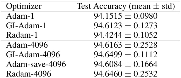
🔼 This table compares the test accuracy achieved by different optimizers (Adam, GI-Adam, Radam) with different warmup durations (1 and 4096 steps). The results demonstrate how the choice of optimizer and warmup duration affects the final performance of the model. The ‘Adam-save’ row indicates a modified warmup strategy to improve efficiency.
read the caption
Table 1: Performance comparison of different optimizers with varying warmup durations.
Full paper#
