↗ OpenReview ↗ NeurIPS Homepage ↗ Chat
TL;DR#
Deep learning model training is resource-intensive due to the increasing complexity and scale of parameters. Existing methods for creating new models typically involve retraining, which is time-consuming and computationally expensive. This paper proposes a paradigm shift by drawing inspiration from the biological visual system, proposing Model Disassembling and Assembling (MDA) to bypass retraining.
MDA introduces techniques for disassembling trained CNN classifiers into task-aware components, using concepts like relative contribution and component locating. It then presents strategies for reassembling these components into new models tailored for specific tasks, utilizing alignment padding and parameter scaling. Experiments show that MDA achieves performance comparable to, or exceeding, baseline models, showcasing its potential for model reuse, compression, and knowledge distillation.
Key Takeaways#
Why does it matter?#
This paper is significant because it introduces a novel and efficient method for creating and reusing deep learning models without retraining. This addresses the growing resource intensiveness of training large models and opens new avenues for model compression, knowledge distillation, and model explanation. The LEGO-like approach to model building simplifies model creation and reuse, making deep learning more accessible to researchers.
Visual Insights#

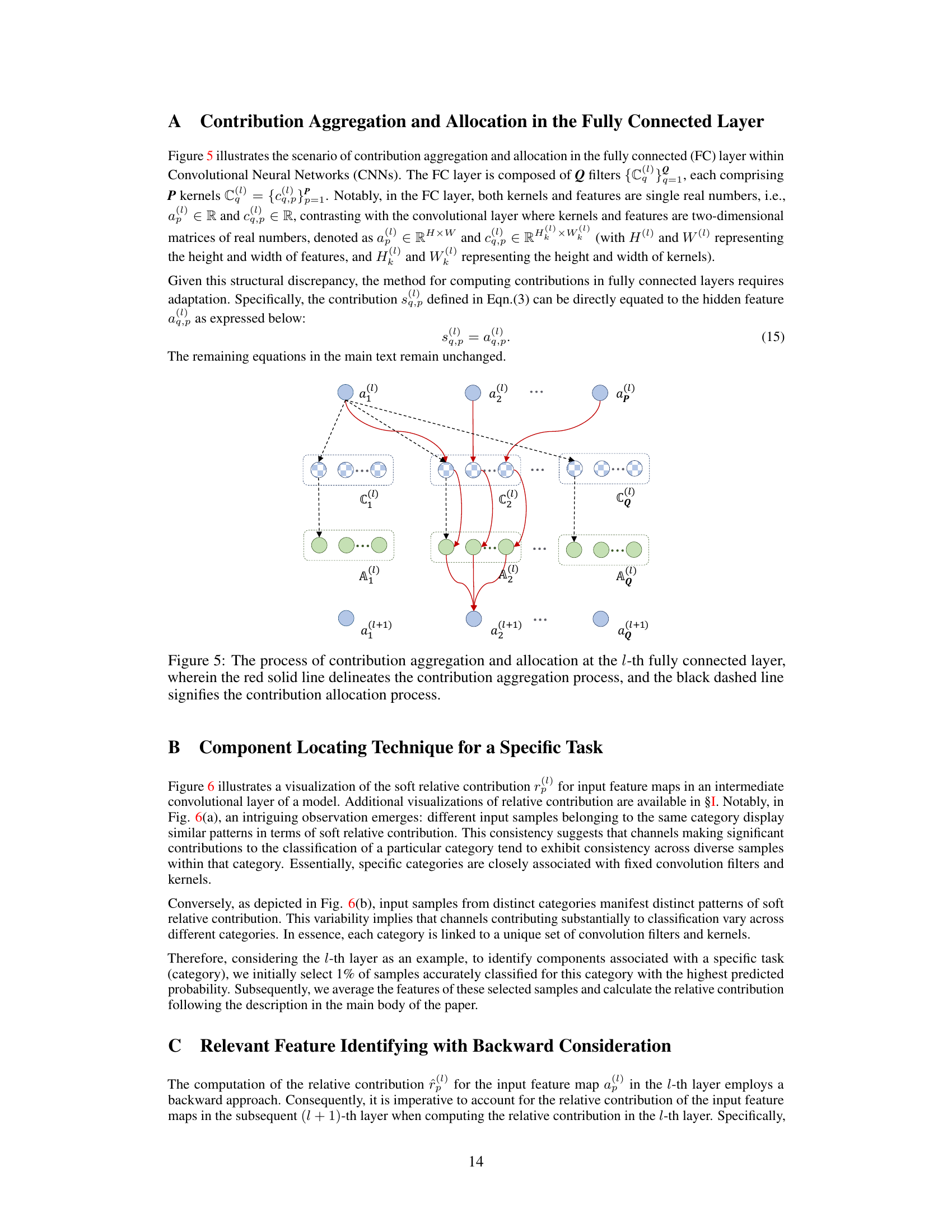
This figure illustrates the process of disassembling a Convolutional Neural Network (CNN) at a specific layer (the l-th layer). The red lines show how contributions from input feature maps are aggregated to hidden feature maps via convolution filters. The black dashed lines illustrate how these contributions are then allocated to various hidden feature maps through different convolution kernels. This process helps in identifying the parameters most relevant to a specific task within the CNN.
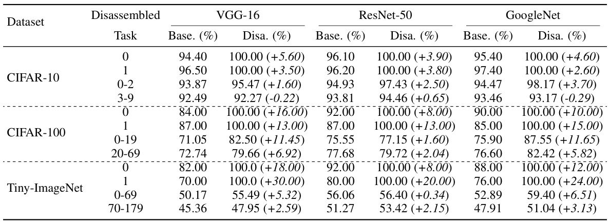
This table presents the results of the model disassembling experiments. It compares the accuracy of the original (‘Base’) model with the accuracy of models created by disassembling task-aware components (‘Disa.’) from the original model. The improvement in accuracy is also shown. The experiments were performed using VGG-16, ResNet-50, and GoogleNet models on three different datasets (CIFAR-10, CIFAR-100, Tiny-ImageNet). Each dataset had multiple tasks (categories) to test.
In-depth insights#
Model LEGO#
The heading ‘Model LEGO’ cleverly encapsulates the core concept of the research paper: creating and reusing deep learning models in a modular and flexible manner. It draws a compelling analogy to LEGO bricks, where pre-trained components (akin to LEGO bricks) are disassembled from existing models and reassembled to build new models tailored to specific tasks. This approach offers several advantages. Firstly, it reduces the resource-intensive process of training new models from scratch. Secondly, it allows for efficient model reuse and adaptation, making deep learning more accessible. Thirdly, the LEGO metaphor emphasizes the interpretability and modularity of the system, fostering a deeper understanding of model behavior and functionality. Finally, this innovative paradigm opens up exciting avenues for model compression, knowledge distillation, and decision route analysis, highlighting the potential of this ‘Model LEGO’ approach to transform the landscape of deep learning model development and deployment.
MDA Method#
The Model Disassembling and Assembling (MDA) method, inspired by biological visual system pathways, offers a novel approach to creating deep learning models without training. MDA leverages the concept of relative contribution to identify task-aware components within pre-trained CNNs. These components, akin to LEGO bricks, are extracted via a component locating technique that considers the relative influence of features on the final prediction. A key innovation is the alignment padding and parameter scaling strategies used to seamlessly assemble these components into new models for specific tasks. This paradigm shift allows for model reuse and creation, offering opportunities for model compression, knowledge distillation, and decision route analysis. The method’s flexibility extends beyond CNNs, with potential applications across various DNN architectures, suggesting a paradigm shift in how we design and utilize deep learning models. Extensive experimental validation demonstrates the efficacy of MDA, with assembled models often matching or exceeding the performance of baseline models, highlighting its potential to transform model development.
MDA Results#
An in-depth analysis of MDA results would require access to the full research paper. However, we can anticipate that such a section would present quantitative evidence supporting the core claims of the paper. Key metrics like accuracy, precision, and recall for different tasks and model architectures would likely be reported. Comparisons to baseline models (without MDA) are crucial to demonstrate the effectiveness of the proposed technique. Results might be presented across various datasets to highlight generalizability and robustness. Additionally, visualizations could effectively illustrate the differences between models created with and without MDA, offering an intuitive understanding of the results. A thorough analysis would delve into specific findings across all experiments showing how task-aware components perform when combined and their impact on model size and computational efficiency. The results section should highlight both successful and unsuccessful aspects of the MDA process, helping readers assess limitations and guide future work.
Future Work#
The authors acknowledge limitations in their current Model Disassembling and Assembling (MDA) approach, particularly concerning the accuracy decline observed in certain multi-task assembling scenarios. Future work will focus on mitigating the negative impact of irrelevant components during model assembly, enhancing the method’s robustness and stability. The current study concentrates on CNN classifiers; future research will explore MDA’s application to other network architectures, such as object detection and segmentation models, and potentially to other domains like natural language processing. A crucial aspect for future investigation is improving the efficiency and scalability of the MDA framework. This includes exploring methods to reduce computational costs and improve performance on larger-scale datasets. Further analysis will be done into the factors influencing accuracy and explore techniques to reduce interference between different components within the assembled models. The potential for expanding MDA’s functionality beyond model reuse is also highlighted, for example, to improve model interpretability and to facilitate model compression strategies.
Limitations#
A critical analysis of the limitations section in a research paper is crucial for a comprehensive evaluation. Acknowledging limitations demonstrates intellectual honesty and strengthens the credibility of the research. Areas to examine within a limitations section include: the scope of the study (e.g., specific datasets used, limited sample size), generalizability of findings (can the results be extrapolated to other contexts?), methodological constraints (e.g., limitations of the chosen model or algorithms, biases in data collection), and potential confounding variables. A robust limitations discussion should go beyond merely stating the limitations; it should also offer insights into the implications of these limitations on the study’s overall findings and suggest avenues for future research to address these shortcomings. A well-written limitations section is a hallmark of rigorous scholarship, showcasing that the authors understand the scope and boundaries of their research. Failing to adequately address limitations significantly weakens the paper’s impact, diminishing its contribution to the field.
More visual insights#
More on figures
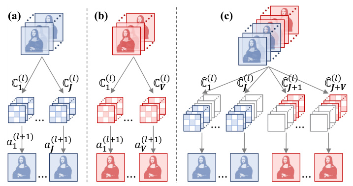
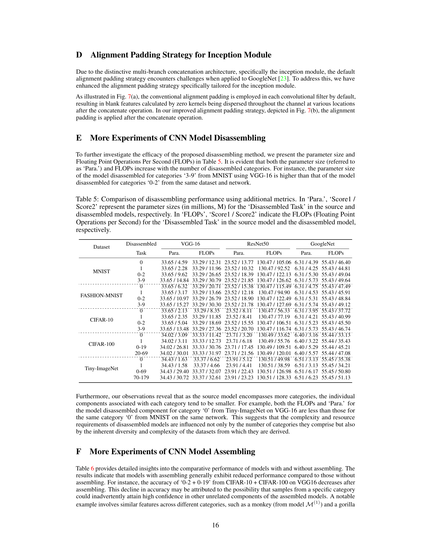
This figure illustrates the process of assembling CNN models layer by layer. Panels (a) and (b) show two different disassembled models, each with a different number of kernels in their filters. Panel (c) demonstrates how these models are combined using the alignment padding strategy, where empty kernels are added to ensure that all filters in the assembled model have a uniform number of kernels, ensuring a standardized structure for further processing.

This figure shows the impact of hyperparameters α and β on the performance of the disassembled model. The hyperparameters α and β control the threshold for determining which parameters are most relevant to a given task. The plots show that as the hyperparameter values increase, the accuracy decreases, while the FLOPs and parameter size also decrease. The effect of changing α and β is more pronounced in the convolutional layers compared to the fully connected layers.
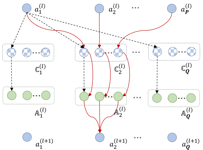
This figure illustrates the process of disassembling a Convolutional Neural Network (CNN) at a given layer (l). The red lines show how the contributions from input feature maps are aggregated to produce hidden feature maps. The black dashed lines show how those contributions are allocated to different convolutional kernels in that layer. This process is a key part of the Model Disassembling and Assembling (MDA) method, which aims to extract task-aware components from a trained CNN.

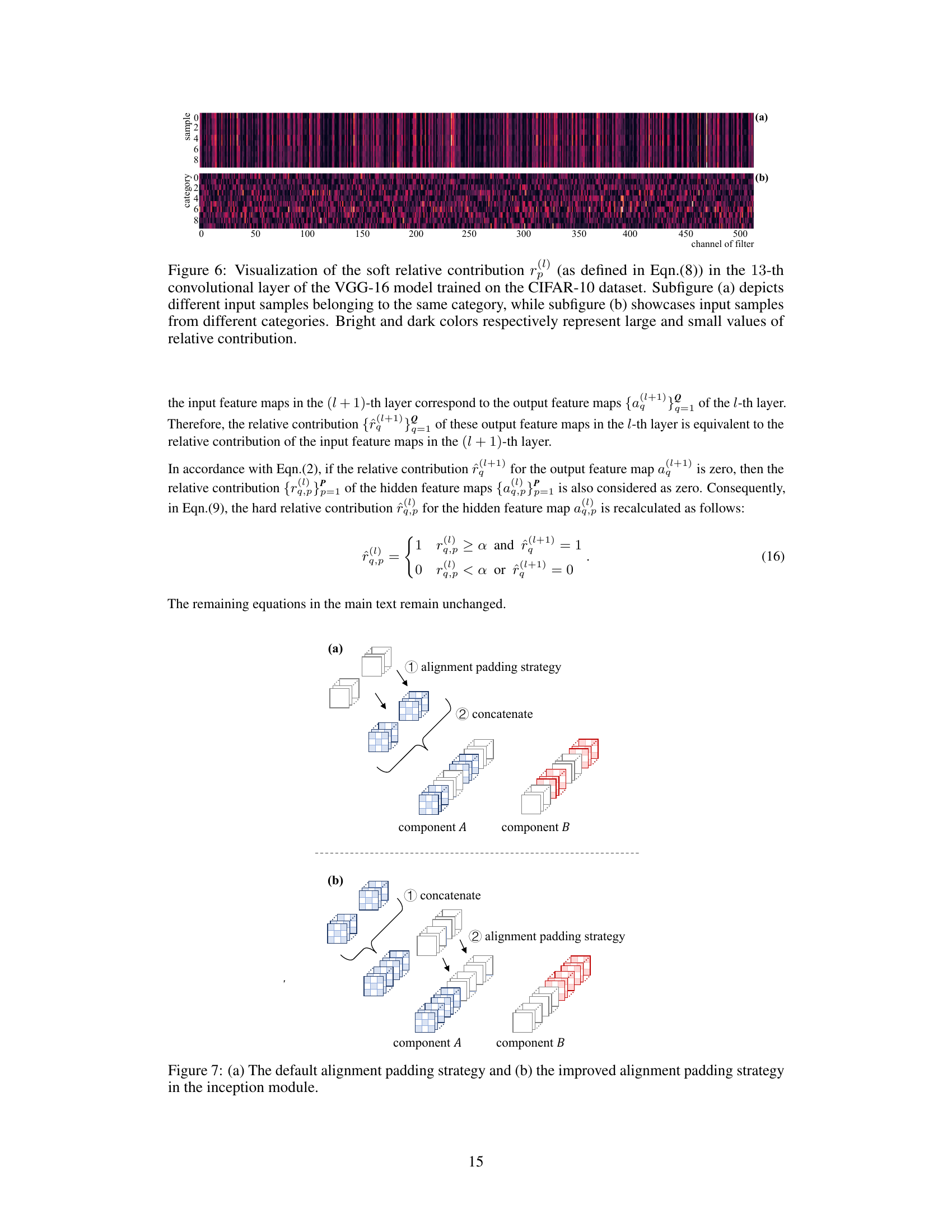
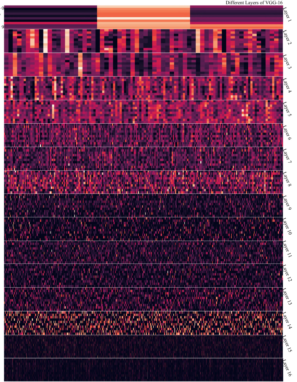
This figure visualizes the relative contribution of input features to the output of the 13th convolutional layer in a VGG-16 model trained on CIFAR-10. (a) shows that inputs from the same category have similar contribution patterns. (b) demonstrates that inputs from different categories have distinct contribution patterns, highlighting the task-specific nature of these contributions.
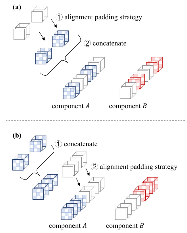
This figure illustrates the process of assembling CNN models layer by layer. It shows how disassembled models (a and b), each with a different number of filters (kernels), are combined. The alignment padding strategy is used to make the number of kernels uniform in the combined layer (c), ensuring compatibility during assembly. The process involves padding empty kernels to each filter to ensure that all filters in a given layer have the same number of kernels.
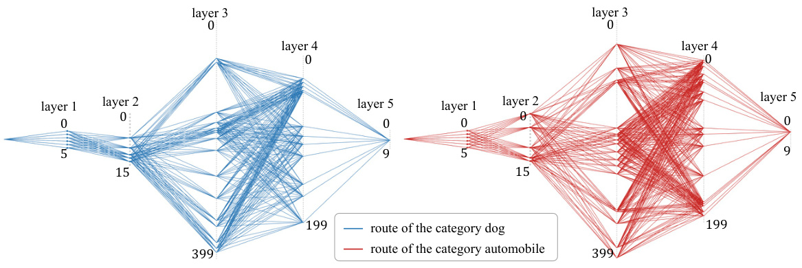
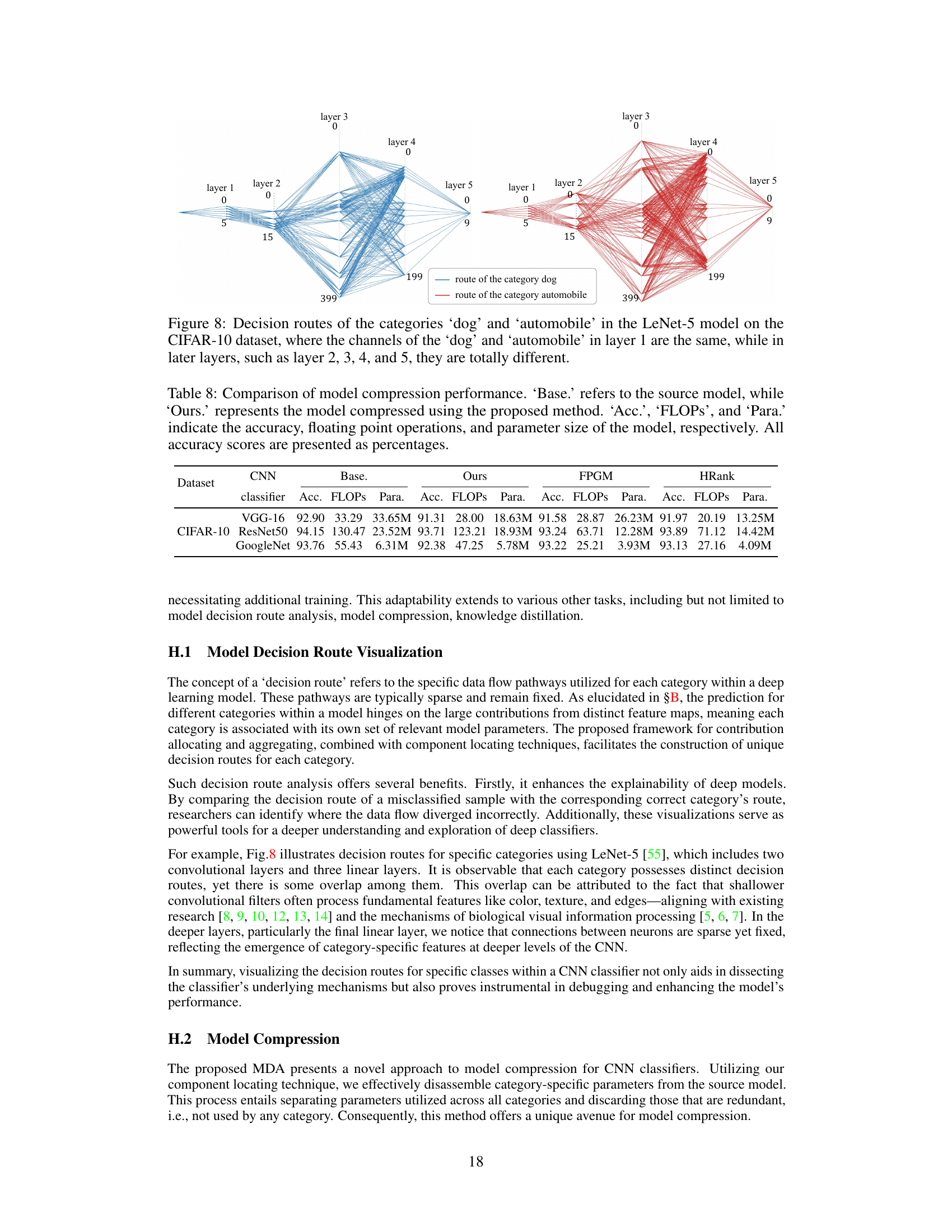
This figure visualizes the decision routes for the categories ‘dog’ and ‘automobile’ within the LeNet-5 model trained on the CIFAR-10 dataset. It demonstrates how the pathways of activation through the network differ significantly between these two categories, even though they share some common channels in the initial layers. The differences in pathways highlight how the model distinguishes between these categories by processing different features at different stages of the network.
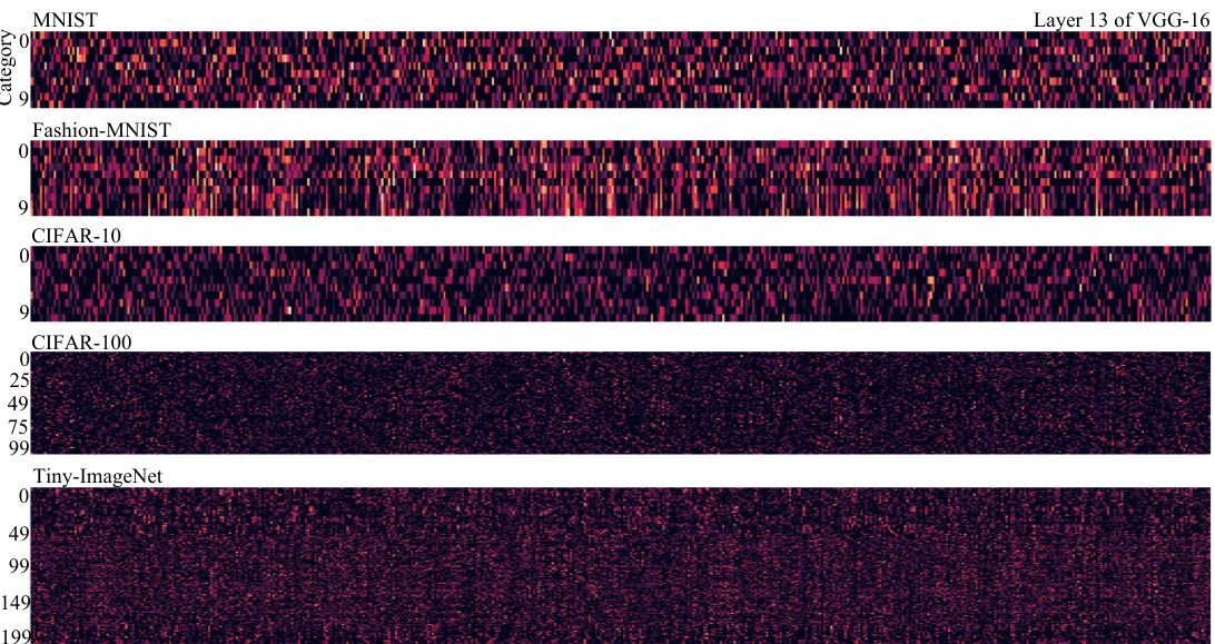
This figure visualizes the soft relative contribution for input samples from various categories in layer 13 of the VGG-16 model, trained on different datasets (MNIST, Fashion-MNIST, CIFAR-10, CIFAR-100, and Tiny-ImageNet). Each row represents a different dataset, and the columns represent different categories within that dataset. The color intensity represents the magnitude of the soft relative contribution, with brighter colors indicating higher contribution values. The visualization helps illustrate the varying levels of contribution different input features make towards the classification of distinct categories in different datasets, offering insight into how different datasets affect feature relevance in different layers of the CNN model.
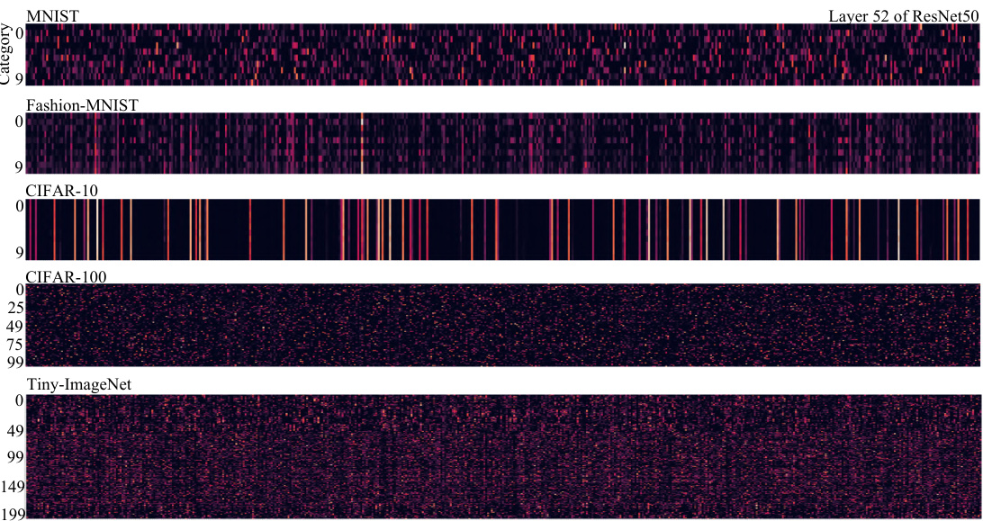
This figure visualizes the soft relative contribution of input features to different categories in layer 52 of a ResNet50 model trained on several datasets (MNIST, Fashion-MNIST, CIFAR-10, CIFAR-100, Tiny-ImageNet). Each row represents a different dataset, and each column represents a different category within that dataset. The color intensity reflects the magnitude of the contribution, with brighter colors indicating stronger contributions.

This figure visualizes the soft relative contribution for input samples from different categories in layer 66 of the GoogleNet model, trained on various datasets. Each row represents a different dataset (MNIST, Fashion-MNIST, CIFAR-10, CIFAR-100, Tiny-ImageNet), and within each row, different color intensities represent the relative contribution of different channels to the classification of a specific category. Darker colors represent smaller contributions, while brighter colors represent larger contributions. This visualization helps illustrate how different channels contribute differently across different datasets and categories.
This figure illustrates the process of disassembling a CNN model at a particular layer (l). The red lines show how the contributions from input feature maps are aggregated to the hidden feature maps using a convolutional filter. The black dashed lines demonstrate how these aggregated contributions are then allocated to the different hidden feature maps. This process is crucial for identifying the components of the CNN model that are most relevant to specific tasks.
More on tables
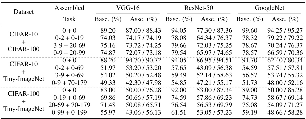
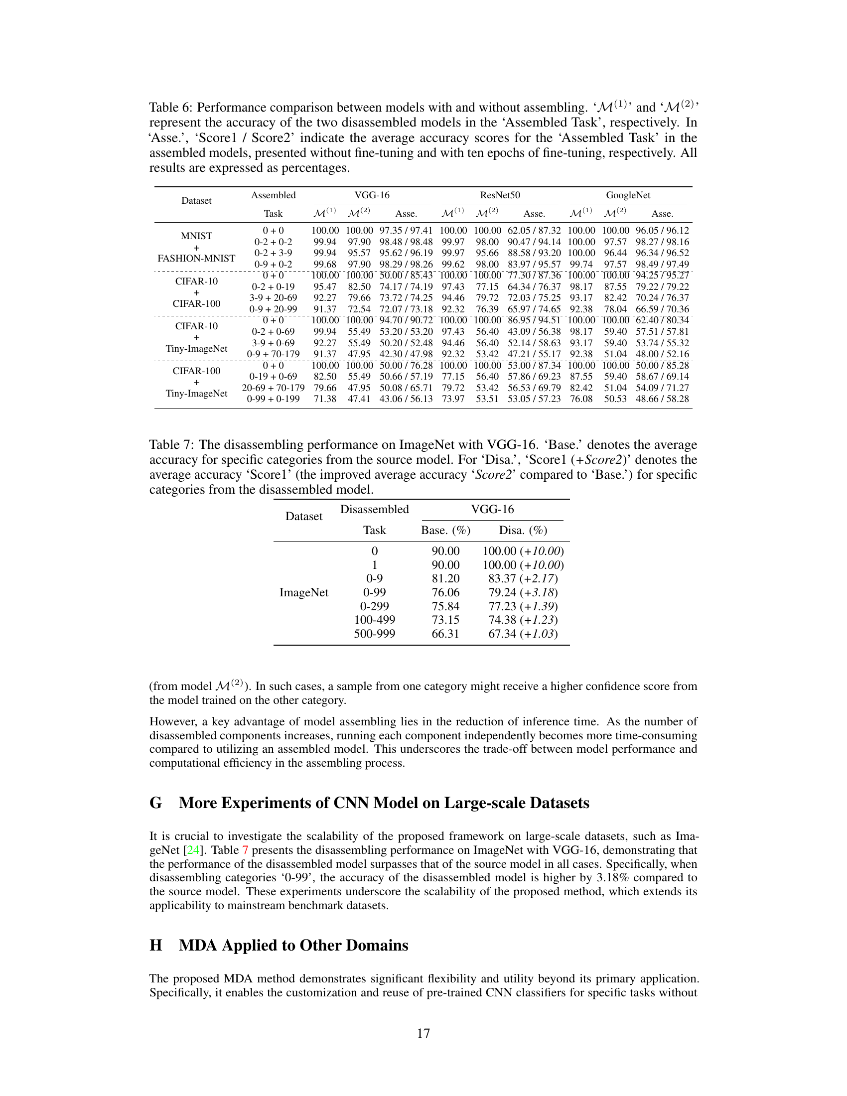
This table presents the results of the model assembling experiments. It compares the average accuracy of the assembled models (‘Asse.’) to the baseline accuracy (‘Base.’) of the source models for various assembled tasks across different datasets (CIFAR-10, CIFAR-100, and Tiny-ImageNet). The ‘Asse.’ column shows two scores: ‘Score1’ represents the accuracy without any fine-tuning after assembling, and ‘Score2’ represents the accuracy after ten epochs of fine-tuning.
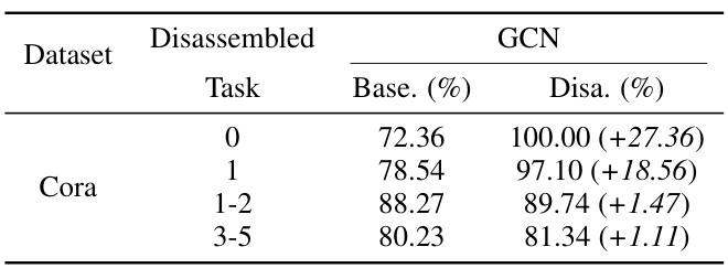
This table presents the results of applying the Model Disassembling and Assembling (MDA) method to a Graph Convolutional Network (GCN) model for node classification on the Cora dataset. It compares the average accuracy (‘Base.’) of the original GCN model for specific tasks (categories 0, 1, 1-2, and 3-5) with the accuracy (‘Disa.’) achieved after disassembling the model using the MDA method. The improvement in accuracy is also shown for each task.

This table compares the performance of different model assembling strategies. The ‘Base’ column shows the average accuracy of the assembled task in the source models. The ‘+Padd.’ column presents the accuracy when only the alignment padding strategy is used, while the ‘+Padd. +Para.’ column shows the accuracy when both alignment padding and parameter scaling strategies are applied. The results highlight the impact of both strategies on the final accuracy of the assembled model.
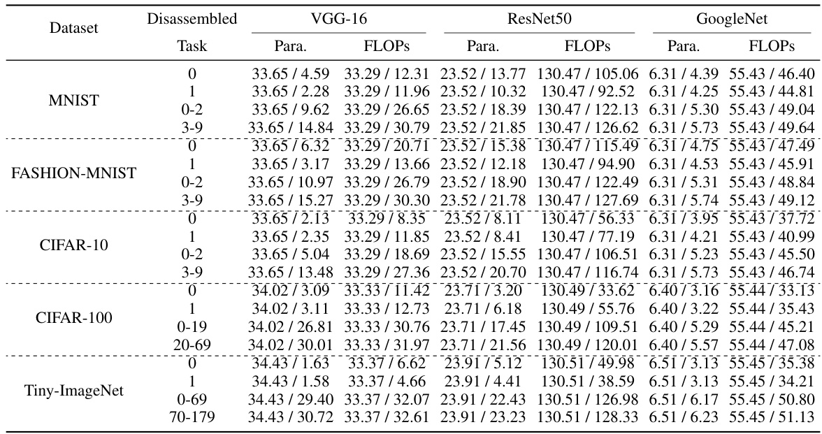
This table presents the results of the model disassembling experiments. It compares the performance of the original model (‘Base’) against the performance after disassembling task-aware components (‘Disa’). For each task (represented by a category in the classification problem), the table shows the base accuracy, the accuracy after disassembling, and the improvement in accuracy resulting from the disassembling process. The dataset used is specified in the first column.
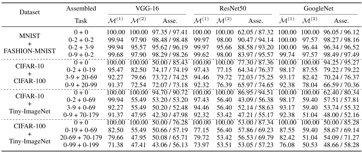
This table presents the results of the model assembling process. It compares the average accuracy of the assembled models (‘Asse.’) to the baseline accuracy from the source models (‘Base.’) for various assembled tasks on different datasets. The accuracy is reported with and without fine-tuning (10 epochs). The ‘Score1’ represents the accuracy without fine-tuning, and ‘Score2’ the accuracy with fine-tuning (10 epochs).
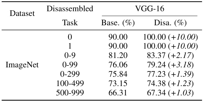
This table presents the results of the model disassembling experiments. It compares the average accuracy (‘Base.’) of a given task (category) in the original trained model to the accuracy (‘Disa.’) achieved after disassembling that task into a separate, smaller model. The improvement in accuracy (‘Score2’) is also shown, indicating how much better (or worse) the disassembled model performed compared to the original. The experiments were conducted on multiple datasets (CIFAR-10, CIFAR-100, Tiny-ImageNet) and with several different CNN architectures (VGG-16, ResNet-50, GoogleNet).

This table compares the performance of three different model compression methods: the proposed MDA method, FPGM, and HRank. It shows the accuracy, FLOPs (floating point operations), and the number of parameters for each method on three different CNN models (VGG-16, ResNet50, and GoogleNet) trained on the CIFAR-10 dataset. The goal is to demonstrate the trade-offs between compression level and accuracy.
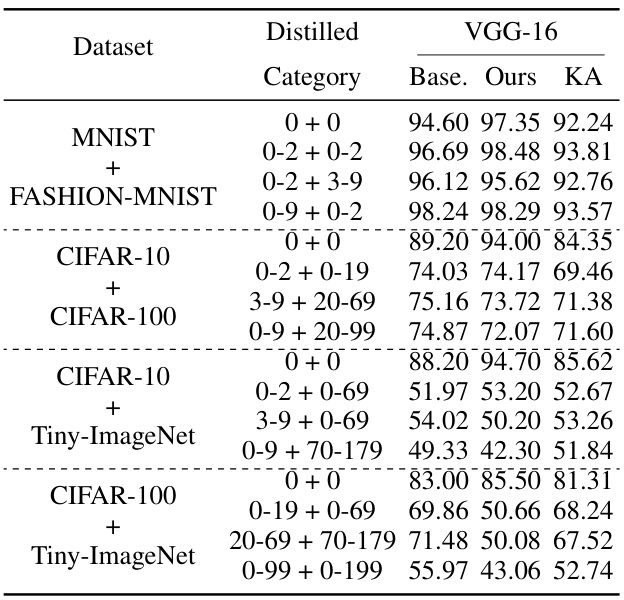
This table presents the results of the model disassembling experiments. It compares the performance of the original model (‘Base.’) with the performance of the model after disassembling (‘Disa.’) for various tasks (categories) on different datasets. The ‘Disa.’ column shows the accuracy of the disassembled model (‘Score1’) and the improvement in accuracy compared to the original model (‘Score2’).
Full paper#
