TL;DR#
Multiparameter persistent homology is a powerful tool for analyzing complex datasets, but existing methods for summarizing this information are often computationally expensive and difficult to interpret. This poses a significant challenge for researchers seeking to integrate topological insights into machine learning workflows. Existing methods also often rely on transforming topological summaries into high-dimensional vectors, which can be computationally expensive and may lose some important information.
This paper introduces “graphcodes”, a novel method for summarizing multiparameter persistent homology that addresses these limitations. Graphcodes represent the topological information as an embedded graph, which can be efficiently computed and readily integrated into machine learning pipelines using graph neural networks. The authors demonstrate that graphcodes outperform existing methods on various datasets in terms of both accuracy and computational efficiency.
Key Takeaways#
Why does it matter?#
This paper is important because it introduces a novel method for summarizing multiparameter persistent homology, which is a crucial tool for understanding the topological structure of complex datasets. The proposed method, called “graphcodes”, offers several advantages over existing techniques, including efficiency, interpretability, and direct integration with machine learning pipelines using graph neural networks. This work is relevant to researchers working in topological data analysis, machine learning, and related fields because it provides a practical solution to a long-standing challenge and opens up new avenues for research.
Visual Insights#

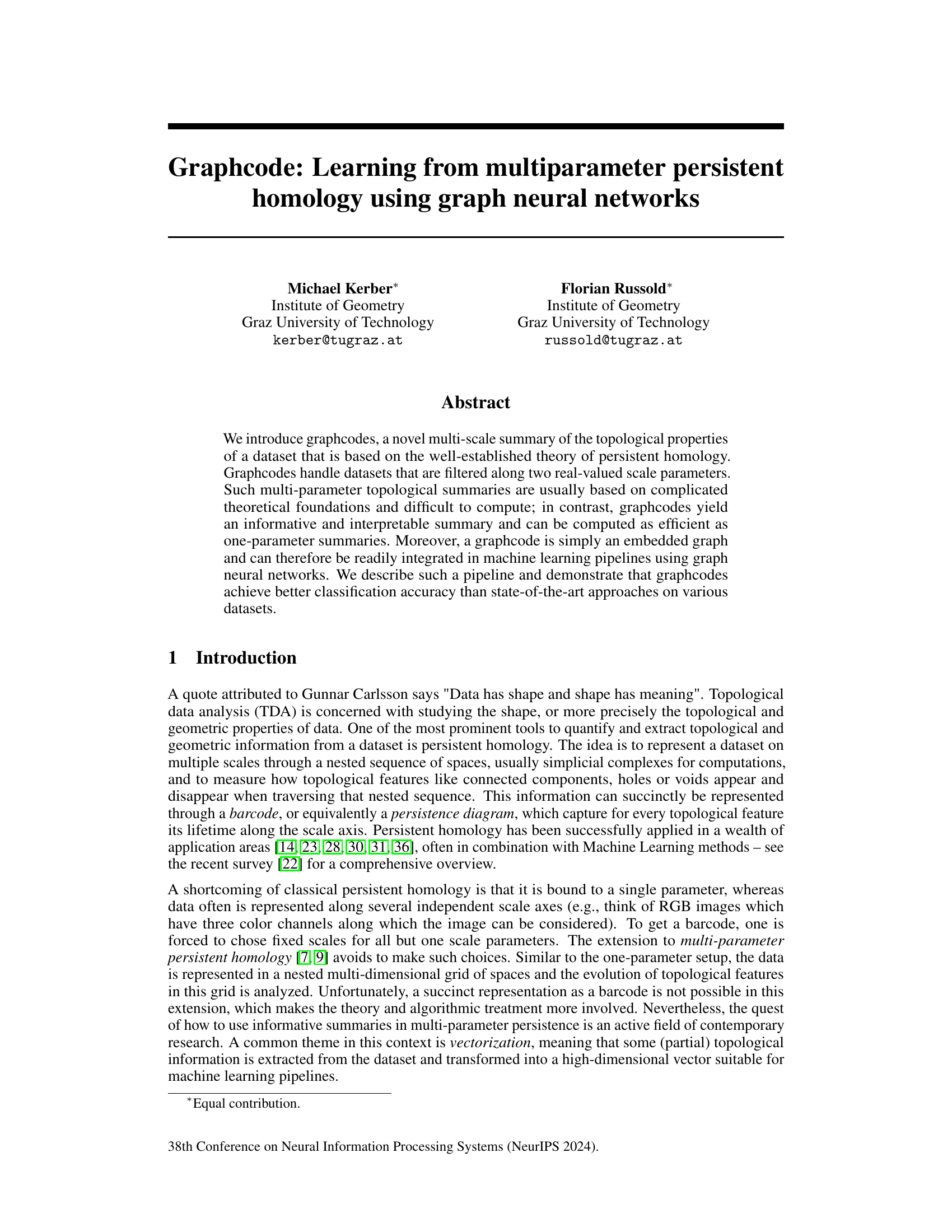
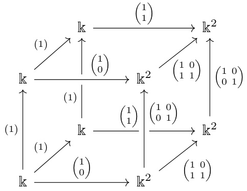
🔼 This figure illustrates the process of creating graphcodes from a dataset. The dataset is filtered along two scale parameters, resulting in a bifiltration (a stack of nested simplicial complexes). For each fixed parameter value, we compute a one-parameter persistent homology, yielding persistence diagrams. These diagrams are then connected through maps induced by homology maps between the nested simplicial complexes, forming bipartite graphs between consecutive pairs. The union of these bipartite graphs forms the graphcode, a multi-scale summary of the dataset’s topology.
read the caption
Figure 1: Schematic overview of our approach.

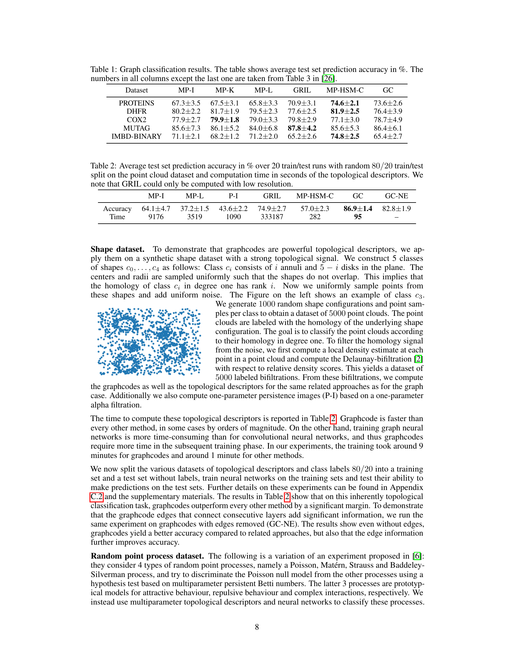
🔼 This table presents the results of graph classification experiments using various multi-parameter persistent homology methods. It compares the performance of Graphcodes (GC) against several state-of-the-art techniques (MP-I, MP-K, MP-L, GRIL, MP-HSM-C) across five different graph datasets (PROTEINS, DHFR, COX2, MUTAG, IMDB-BINARY). The accuracy (in percentage) is reported for each method and dataset, providing a comparative analysis of their effectiveness in graph classification tasks. Note that the accuracy values for methods other than GC are taken from a previous study referenced as [26].
read the caption
Table 1: Graph classification results. The table shows average test set prediction accuracy in %. The numbers in all columns except the last one are taken from Table 3 in [26].
In-depth insights#
Multiparameter TDA#
Multiparameter topological data analysis (TDA) extends the capabilities of traditional TDA by considering datasets filtered along multiple parameters, instead of just one. This is crucial for analyzing complex data with inherent multi-scale structure, such as images (RGB channels) or time series with multiple features. A key challenge in multiparameter TDA is the complexity of summarizing the resulting multi-dimensional persistence information. Unlike the convenient barcodes of single-parameter TDA, multiparameter persistence lacks a concise, easily interpretable visualization. This necessitates the development of sophisticated summary methods. The paper explores graphcodes, a novel method to represent multiparameter persistence. Graphcodes are computationally efficient and readily integrated into machine learning workflows through their graph representation. By efficiently summarizing the topological information, they provide an alternative to more computationally expensive vectorization techniques common in multiparameter TDA. The effectiveness of graphcodes is demonstrated via classification experiments, highlighting their potential as a valuable tool in the analysis and machine learning of multi-parameter data.
Graph Neural Nets#
The application of Graph Neural Networks (GNNs) to process graphcodes, novel topological summaries of multi-parameter persistent homology, represents a significant advancement. GNNs’ inherent ability to handle graph-structured data makes them well-suited for this task. Instead of transforming topological information into vectors—a common, less efficient approach—the authors directly feed graphcodes (represented as embedded graphs) into the GNN. This pipeline avoids information loss inherent in vectorization and potentially achieves higher classification accuracy. The choice of GNN architecture is crucial, with the paper utilizing Graph Attention Networks (GATs) to focus on high-persistence features. The described pipeline is both efficient and effective, demonstrating the strength of this novel approach. The architecture uses multiple GAT layers followed by a max-pooling step for each slice of the bifiltration, and finally a dense layer for classification, suggesting a flexible and potentially adaptable framework for various topological data analysis tasks.
GraphCode Encoding#
GraphCode encoding offers a novel approach to summarizing topological information from multiparameter persistent homology. Instead of relying on computationally expensive vectorizations of persistence diagrams, GraphCodes leverage graph neural networks for direct processing of topological data. By representing the data as a graph, where nodes correspond to topological features and edges capture their relationships across multiple scales, GraphCodes enable efficient computation and integration with machine learning pipelines. This approach avoids information loss associated with existing vectorization techniques, leading to potentially improved classification accuracy. The efficiency stems from a clever algorithm based on out-of-order matrix reduction, significantly reducing computational cost compared to alternative methods. While not a topological invariant due to basis dependence, the interpretability and performance of GraphCodes on various datasets suggest its practical value for topological data analysis.
Computational Limits#
A hypothetical section titled ‘Computational Limits’ in a research paper on topological data analysis would likely explore the computational challenges inherent in calculating persistent homology, especially for high-dimensional data or complex filtrations. The analysis would probably discuss the complexity of algorithms for computing persistent homology, perhaps focusing on the computational cost of matrix reduction and other key steps. Scalability issues when dealing with large datasets would be examined, along with potential bottlenecks and limitations. The discussion might cover memory usage, runtime, and how these factors affect the practicality of applying TDA to various applications. It would also likely address the trade-offs between accuracy and computational efficiency—simplified algorithms might reduce runtime but sacrifice accuracy, and vice versa. Finally, the section could propose or discuss approaches to mitigate these computational limitations, such as using approximation methods, parallel processing, or specialized hardware. This section would be crucial to providing a realistic assessment of the applicability and limitations of the presented topological methods.
Future Extensions#
Future research directions could explore adapting graphcodes for different data types beyond point clouds and graphs, such as images or time series. Investigating alternative methods for basis selection in graphcode construction, potentially leveraging machine learning techniques, could enhance reproducibility and topological invariance. A promising area is combining graphcodes with more sophisticated graph neural network architectures to improve classification accuracy and scalability. Finally, exploring the theoretical properties of graphcodes, such as their stability under noise or perturbations, is crucial for building confidence in their reliability and robustness as a general-purpose topological descriptor. This would involve rigorous mathematical analysis and simulations.
More visual insights#
More on figures
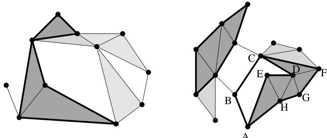
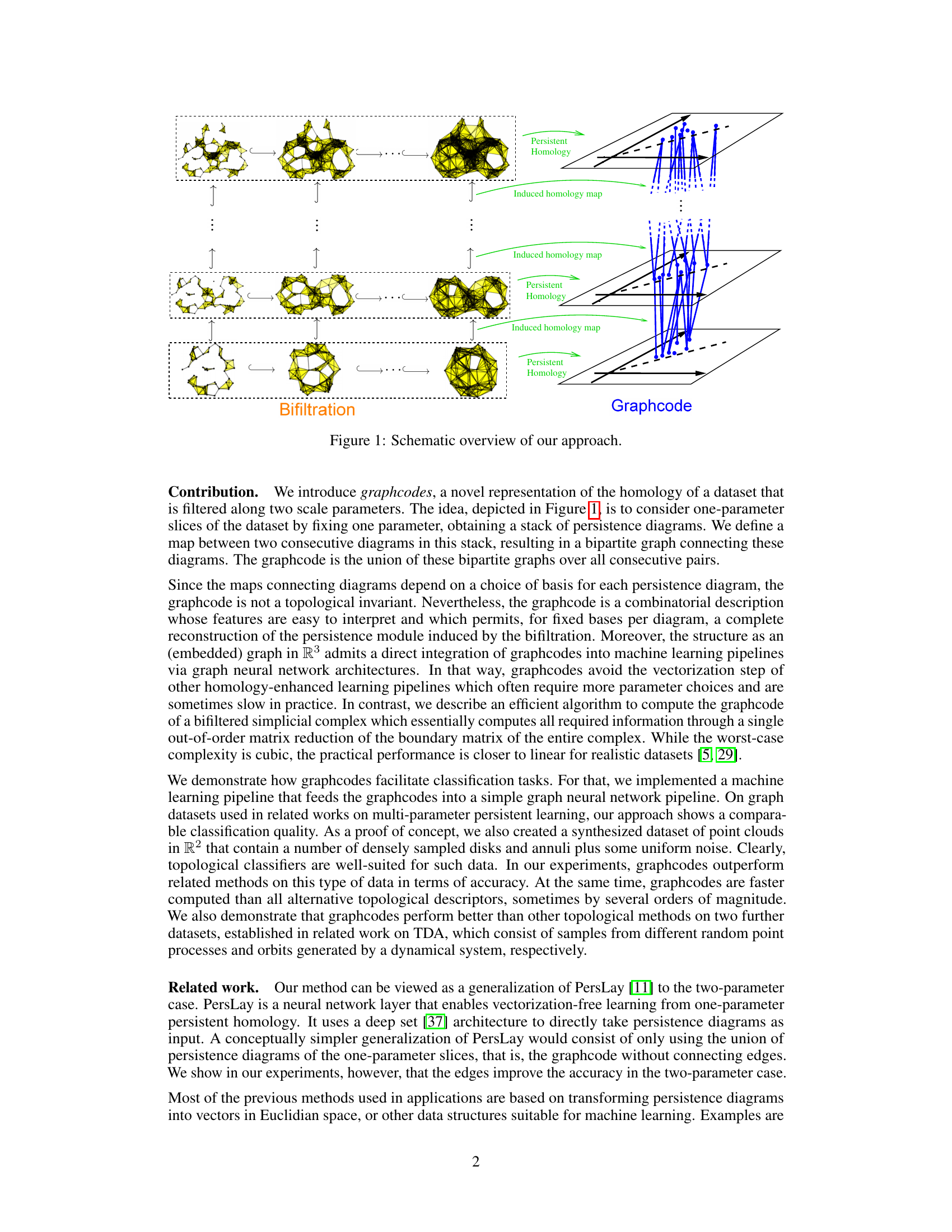
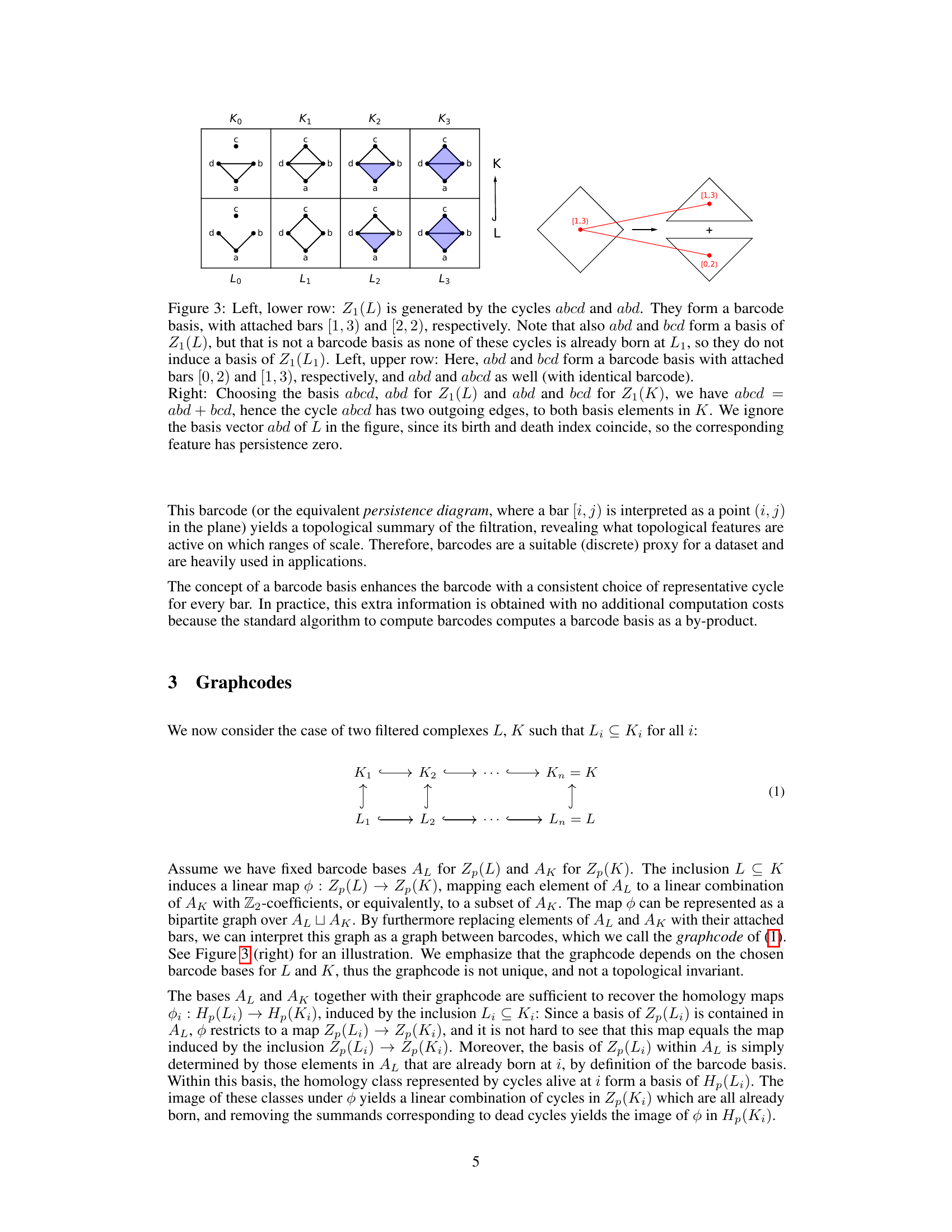
🔼 The figure shows two illustrations related to simplicial complexes and homology. The left side depicts a simplicial complex with its simplices (vertices, edges, and triangles). A 2-chain (a collection of 2-simplices) and its boundary (a 1-cycle) are highlighted. The right side illustrates the concept of homology classes. Two 1-cycles (a and a’) are shown, both representing the same homology class because their sum is a 1-boundary.
read the caption
Figure 2: Left: A simplicial complex with 11 0-simplices, 19 1-simplices and 7 2-simplices. A 2-chain consisting of three 2-simplices is marked with darker color, and its boundary, a collection of 7 1-simplices is displayed in thick. Right: The 1-cycle marked in thick on the left is also a 1-boundary, since it is the image of the boundary operator under the 4 marked 2-simplices. On the right, the 1-cycle a going along the path ABCDE is not a 1-boundary; therefore it is a generator of an homology class [a] of H₁(K). Likewise, the 1-cycle a' going along ABCFGH is not a 1-boundary neither. Furthermore, [a'] = [a] since the sum a + a' is the 1-cycle given by the path AEDCFGH, which is a 1-boundary because of the 5 marked 2-simplices. Hence, a and a' represent the same homology class which is characterized by looping aroung the same hole in K.

🔼 This figure illustrates the concept of barcode bases and how they relate to persistence diagrams and graphcodes. The left side shows two different barcode bases for the same homology group Z1(L) of a complex L under a filtration, highlighting that a barcode basis is not unique but all yield the same barcode. Bars represent the lifespans of topological features. The right side depicts how a homology map between two complexes L and K, represented as a bipartite graph, connects corresponding bars from their respective barcodes. Edges represent the relationships between these features as the complexes are filtered.
read the caption
Figure 3: Left, lower row: Z1(L) is generated by the cycles abcd and abd. They form a barcode basis, with attached bars [1, 3) and [2, 2), respectively. Note that also abd and bed form a basis of Z1(L), but that is not a barcode basis as none of these cycles is already born at L₁, so they do not induce a basis of Z1(L1). Left, upper row: Here, abd and bcd form a barcode basis with attached bars [0, 2) and [1, 3), respectively, and abd and abcd as well (with identical barcode). Right: Choosing the basis abcd, abd for Z1(L) and abd and bed for Z1(K), we have abcd = abd + bcd, hence the cycle abcd has two outgoing edges, to both basis elements in K. We ignore the basis vector abd of L in the figure, since its birth and death index coincide, so the corresponding feature has persistence zero.

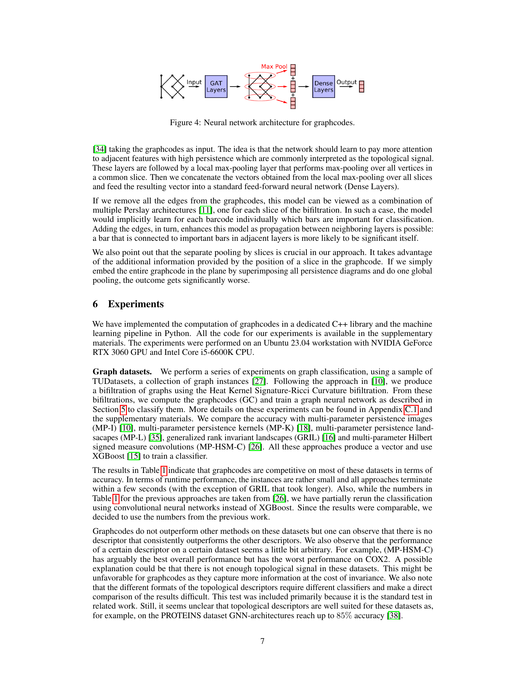
🔼 This figure depicts the neural network architecture used for processing graphcodes. The input is a graphcode (a layered graph representing multi-parameter persistent homology). This graphcode is fed into Graph Attention (GAT) layers, which are designed to handle graph-structured data. The GAT layers are followed by a max-pooling layer applied separately to each layer of the graphcode, extracting important features. The results from each layer’s max-pooling are then concatenated and passed through dense layers. Finally, the dense layers output a classification result.
read the caption
Figure 4: Neural network architecture for graphcodes.
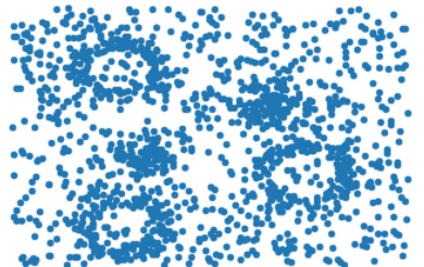
🔼 This figure illustrates the concept of barcode bases and graphcodes using a simple example with two filtered complexes, L and K. The left side shows how a barcode basis (a set of cycles with birth and death times) is chosen from the cycles of L, focusing on consistent bases. The right side illustrates the graphcode construction, showcasing how to represent the homology maps between the complexes using a bipartite graph connecting the bars (intervals) representing homology classes in L and K.
read the caption
Figure 3: Left, lower row: Z1(L) is generated by the cycles abcd and abd. They form a barcode basis, with attached bars [1, 3) and [2, 2), respectively. Note that also abd and bed form a basis of Z1(L), but that is not a barcode basis as none of these cycles is already born at L₁, so they do not induce a basis of Z1(L1). Left, upper row: Here, abd and bcd form a barcode basis with attached bars [0, 2) and [1, 3), respectively, and abd and abcd as well (with identical barcode). Right: Choosing the basis abcd, abd for Z1(L) and abd and bed for Z1(K), we have abcd = abd + bcd, hence the cycle abcd has two outgoing edges, to both basis elements in K. We ignore the basis vector abd of L in the figure, since its birth and death index coincide, so the corresponding feature has persistence zero.
🔼 This figure illustrates the concept of barcode bases and their relation to persistence diagrams. The left side shows two different barcode bases for the same homology group, highlighting that the basis choice affects the representation. The right side demonstrates how a barcode basis in one complex maps to another, visualized as a bipartite graph representing the homology map. This illustrates how the graphcode uses barcode bases to capture the evolution of topological features across different filtration levels.
read the caption
Figure 3: Left, lower row: Z1(L) is generated by the cycles abcd and abd. They form a barcode basis, with attached bars [1, 3) and [2, 2), respectively. Note that also abd and bed form a basis of Z1(L), but that is not a barcode basis as none of these cycles is already born at L₁, so they do not induce a basis of Z1(L1). Left, upper row: Here, abd and bcd form a barcode basis with attached bars [0, 2) and [1, 3), respectively, and abd and abcd as well (with identical barcode). Right: Choosing the basis abcd, abd for Z1(L) and abd and bed for Z1(K), we have abcd ≈ abd + bcd, hence the cycle abcd has two outgoing edges, to both basis elements in K. We ignore the basis vector abd of L in the figure, since its birth and death index coincide, so the corresponding feature has persistence zero.

🔼 This figure illustrates the concept of barcode basis in persistent homology. The left side shows two examples of barcode bases for the same homology group Z1(L) with different sets of basis elements and corresponding bars. The right side demonstrates how the homology map between two simplicial complexes L and K can be represented as a bipartite graph between their barcode bases.
read the caption
Figure 3: Left, lower row: Z1(L) is generated by the cycles abcd and abd. They form a barcode basis, with attached bars [1, 3) and [2, 2), respectively. Note that also abd and bed form a basis of Z1(L), but that is not a barcode basis as none of these cycles is already born at L₁, so they do not induce a basis of Z1(L1). Left, upper row: Here, abd and bcd form a barcode basis with attached bars [0, 2) and [1, 3), respectively, and abd and abcd as well (with identical barcode). Right: Choosing the basis abcd, abd for Z1(L) and abd and bed for Z1(K), we have abcd = abd + bcd, hence the cycle abcd has two outgoing edges, to both basis elements in K. We ignore the basis vector abd of L in the figure, since its birth and death index coincide, so the corresponding feature has persistence zero.
More on tables

🔼 This table presents a comparison of different topological descriptors on a synthetic shape dataset. The ‘Accuracy’ column shows the average classification accuracy achieved by each method across 20 independent runs, with the training and test sets randomly split 80/20 each time. The ‘Time’ column indicates the computation time in seconds for each descriptor. The table highlights the superior accuracy and efficiency of Graphcodes (GC) compared to other state-of-the-art methods, although GRIL’s performance may be underestimated due to low resolution constraints.
read the caption
Table 2: Average test set prediction accuracy in % over 20 train/test runs with random 80/20 train/test split on the point cloud dataset and computation time in seconds of the topological descriptors. We note that GRIL could only be computed with low resolution.

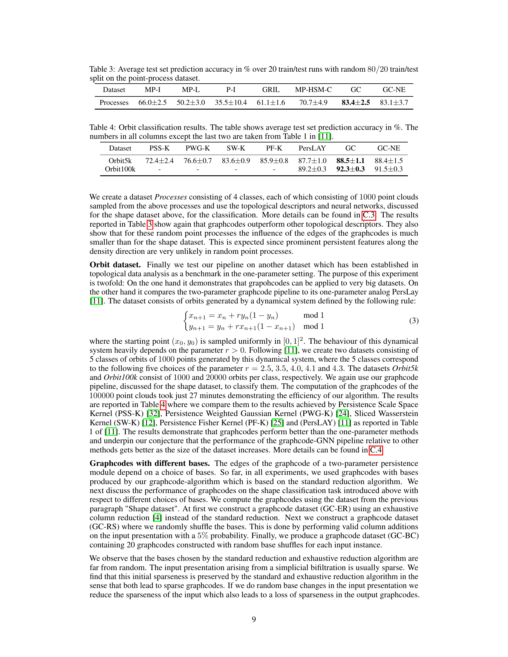
🔼 This table presents the average test set prediction accuracy for different topological descriptors on the point-process dataset. The accuracy is calculated over 20 independent train/test runs with an 80/20 split. The table compares the performance of Graphcodes (GC) and Graphcodes without edges (GC-NE) to other methods like Persistence Images (MP-I), Persistence Landscapes (MP-L), Persistence Images on one parameter (P-I), Generalized Rank Invariant Landscapes (GRIL), and Multi-parameter Hilbert signed measure convolutions (MP-HSM-C).
read the caption
Table 3: Average test set prediction accuracy in % over 20 train/test runs with random 80/20 train/test split on the point-process dataset.

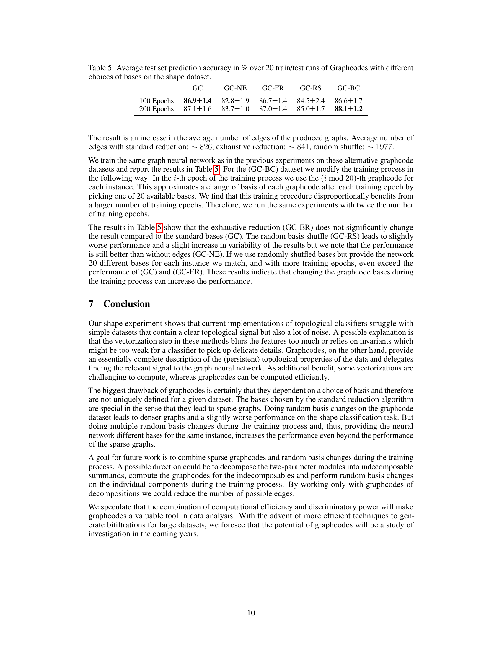
🔼 This table presents the results of orbit classification experiments using different topological methods. It compares the accuracy of several techniques (PSS-K, PWG-K, SW-K, PF-K, PersLAY, GC, and GC-NE) on two datasets: Orbit5k and Orbit100k. The results show the average test set prediction accuracy over multiple runs, highlighting the performance of graphcodes (GC) and graphcodes without edges (GC-NE) compared to existing methods. The values for PSS-K through PF-K and PersLAY are taken from a prior publication ([11]), allowing for a direct comparison.
read the caption
Table 4: Orbit classification results. The table shows average test set prediction accuracy in %. The numbers in all columns except the last two are taken from Table 1 in [11].

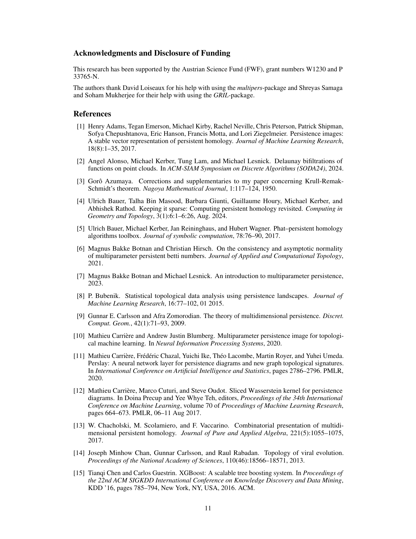
🔼 This table presents the results of experiments evaluating the performance of Graphcodes with different base choices on a shape dataset. The results are averaged over 20 training/testing runs. It compares the accuracy of Graphcodes using standard bases, Graphcodes without edges (GC-NE), Graphcodes using exhaustive reduction for bases (GC-ER), Graphcodes with randomly shuffled bases (GC-RS), and Graphcodes using randomly shuffled bases with a modified training process (GC-BC). The table shows that using randomly shuffled bases, especially with the modified training, improves accuracy compared to standard bases.
read the caption
Table 5: Average test set prediction accuracy in % over 20 train/test runs of Graphcodes with different choices of bases on the shape dataset.
Full paper#
