TL;DR#
Many deep learning models, including Graph Neural Networks (GNNs), suffer from the challenges of vast amounts of data, leading to high computational and memory demands. Data pruning offers a solution by reducing the training data, but existing methods struggle with imbalanced or noisy datasets, often resulting in degraded performance. This paper addresses this issue.
The paper introduces GDeR, a dynamic soft pruning method that uses trainable prototypes to select a representative and balanced subset of the training data during training. This approach not only accelerates training, but also improves the model’s robustness to imbalance and noise, achieving competitive performance with a significantly reduced dataset. Extensive experiments show that GDeR surpasses existing methods in terms of efficiency, balance, and robustness across various datasets and GNN architectures.
Key Takeaways#
Why does it matter?#
This paper is crucial for researchers working with graph neural networks (GNNs) due to its focus on improving training efficiency and robustness. The proposed method, GDeR, offers a practical solution to the challenges of large-scale, imbalanced, and noisy datasets commonly encountered in GNN applications. It opens up new avenues for research into dynamic dataset pruning and graph training debugging, and its applicability extends beyond GNNs, impacting broader AI research.
Visual Insights#

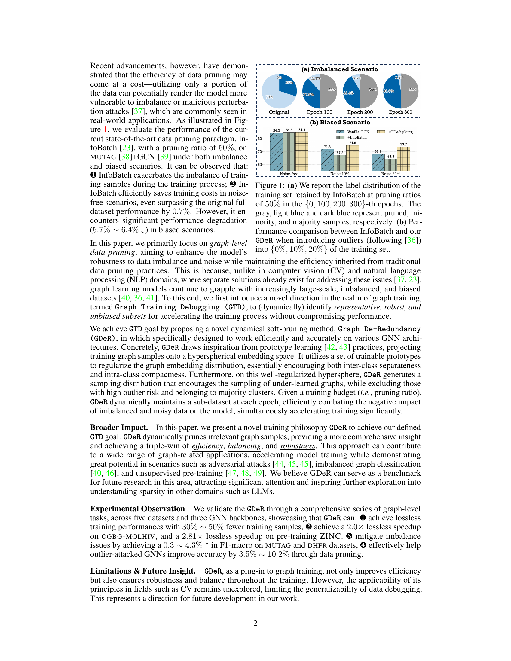
🔼 The figure shows the effect of imbalanced and biased data on the InfoBatch model, a state-of-the-art data pruning method, compared to the proposed GDeR method. In (a), the label distribution of the training set retained by InfoBatch at different epochs with a pruning ratio of 50% is shown, highlighting the imbalance issue. (b) compares the performance of InfoBatch and GDeR under different noise levels (0%, 10%, 20%) added to the training set, demonstrating GDeR’s improved robustness.
read the caption
Figure 1: (a) We report the label distribution of the training set retained by InfoBatch at pruning ratios of 50% in the {0, 100, 200, 300}-th epochs. The gray, light blue and dark blue represent pruned, minority, and majority samples, respectively. (b) Performance comparison between InfoBatch and our GDeR when introducing outliers (following [36]) into {0%, 10%, 20%} of the training set.
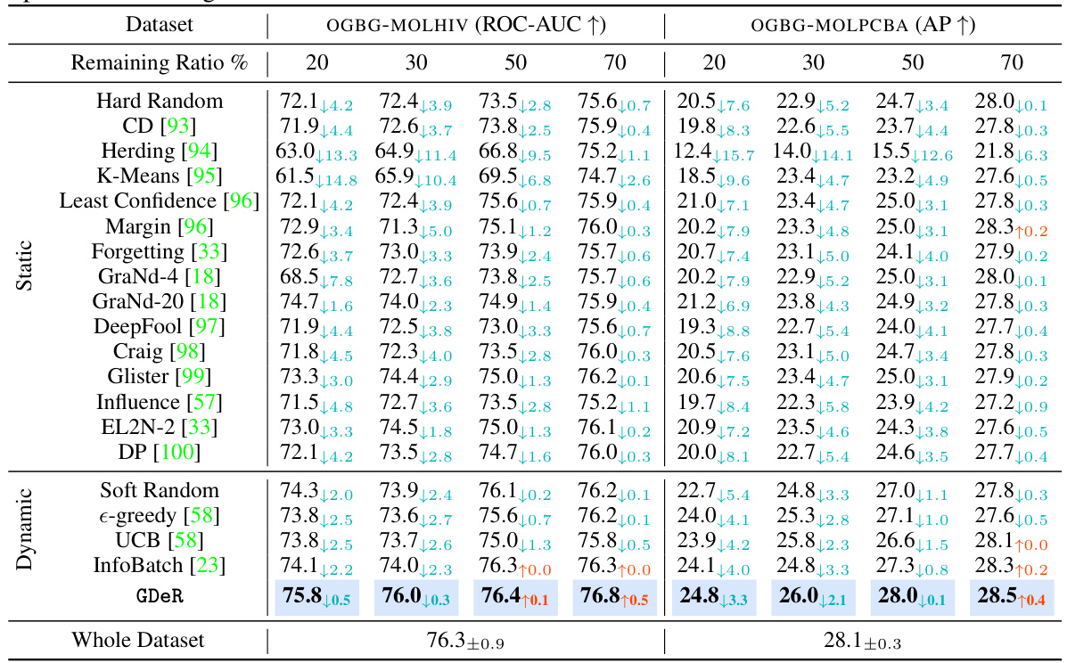
🔼 This table presents a comparison of the performance of various dataset pruning methods, including GDeR, against the full dataset. The methods are tested at different pruning ratios (20%, 30%, 50%, and 70%), with the results averaged over five runs. The performance metric used is ROC-AUC for OGBG-MOLHIV and Average Precision (AP) for OGBG-MOLPCBA. The table shows GDeR’s performance relative to other static and dynamic pruning techniques.
read the caption
Table 1: Performance comparison to state-of-the-art dataset pruning methods when remaining {20%, 30%, 50%, 70%} of the full set. All methods are trained using PNA, and the reported metrics represent the average of five runs.
In-depth insights#
GNN Data Pruning#
GNN data pruning tackles the challenge of training large-scale Graph Neural Networks (GNNs) efficiently by selectively removing less informative or redundant data. This is crucial because GNN training can be computationally expensive, requiring significant resources and time, especially when dealing with massive datasets. The core idea is to identify and retain a subset of the original data that retains crucial information for model training, resulting in faster training without significant performance loss. Different pruning strategies exist, ranging from static methods that pre-process the data before training to dynamic techniques that adapt the pruned dataset during training. The choice of strategy depends on factors such as dataset characteristics, available resources, and the desired trade-off between efficiency and accuracy. Effective GNN data pruning methods strive for balance and robustness, ensuring that the pruned dataset fairly represents the underlying data distribution and avoids performance degradation, particularly when faced with imbalanced or noisy data. A well-designed pruning strategy significantly reduces training time and computational costs while maintaining or even improving the model’s generalization performance. Research in this area is actively developing novel algorithms and techniques to further optimize this balance.
Prototypical GDeR#
The heading ‘Prototypical GDeR’ suggests a method that leverages prototypical learning within the framework of GDeR (Graph De-Redundancy). This implies a system where graph embeddings are projected into a hyperspherical embedding space, and trainable prototypes representing different graph classes are learned within this space. Dynamic sample selection is then guided by these prototypes, prioritizing samples that are poorly represented, imbalanced, or noisy. The use of prototypes offers improved robustness to imbalanced and noisy data, while the dynamic selection optimizes efficiency. The key innovation lies in combining prototype learning’s ability to capture class structures with GDeR’s dynamic pruning for a more efficient and robust training process, addressing the challenges of large-scale graph datasets.
GTD Framework#
A hypothetical “GTD Framework” within a graph-based deep learning context likely involves a systematic process for debugging and improving graph neural network (GNN) training. This would likely incorporate techniques for identifying and addressing issues like data imbalance, noise, and model bias, which commonly hinder GNN performance. The framework’s core would likely center around iterative data pruning or selection, using a principled approach (e.g. prototype-based sampling) to refine the training dataset dynamically. A critical aspect of the framework would be to balance efficiency with robustness, ensuring improved model performance while reducing training times and computational overhead. Further enhancements could include methods for outlier detection and mitigation, potentially incorporating techniques from robust statistics and anomaly detection. The GTD Framework aims to provide a principled, data-centric approach to improve model accuracy and reliability, particularly beneficial in the face of noisy or imbalanced graph-structured data, commonly encountered in real-world applications. Visualization tools could also be integrated to provide insights into the debugging process.
Robustness Gains#
The concept of ‘Robustness Gains’ in the context of a machine learning model, particularly within a graph neural network (GNN) setting, refers to improvements in the model’s performance and reliability when faced with challenging data conditions. This often involves evaluating the model’s ability to handle imbalanced datasets, noisy data points, and even adversarial attacks. Achieving robustness gains is crucial for deploying GNNs in real-world applications where data quality is rarely perfect. Strategies for improving robustness might include data augmentation, regularization techniques, or the development of more resilient model architectures. A key aspect to explore would be the trade-off between robustness and efficiency. Enhanced robustness often comes at the cost of increased computational complexity, so finding methods that provide significant robustness gains without sacrificing efficiency is highly desirable. The evaluation of robustness gains would involve comparing a model’s performance under various challenging conditions against its performance under ideal conditions, demonstrating how effectively the approach mitigates the impact of noise and imbalance. Therefore, a robust model not only achieves high accuracy on clean data but maintains its performance across a range of less-than-ideal data characteristics.
Future of GDeR#
The future of GDeR looks promising, building upon its success in efficient and robust graph training. Extending GDeR’s dynamic pruning capabilities to other data modalities beyond graphs, such as images and text, would broaden its impact significantly. This would require adapting the prototype-based hyperspherical embedding to different data representations, which presents a key challenge and opportunity. Exploring the integration of GDeR with other data augmentation techniques could enhance its ability to handle imbalanced or noisy data, leading to further performance gains. Investigating how to further optimize the prototype selection and updating mechanism to reduce computational cost could improve the speedup achieved. Finally, developing theoretical guarantees for GDeR’s performance would significantly increase its credibility and reliability for broader adoption in machine learning.
More visual insights#
More on figures
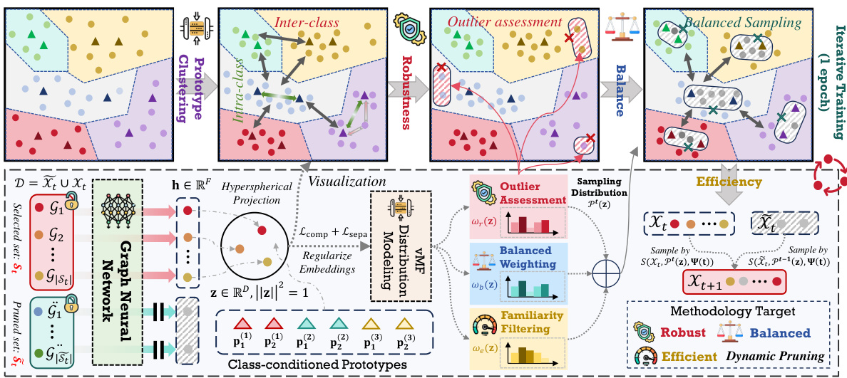
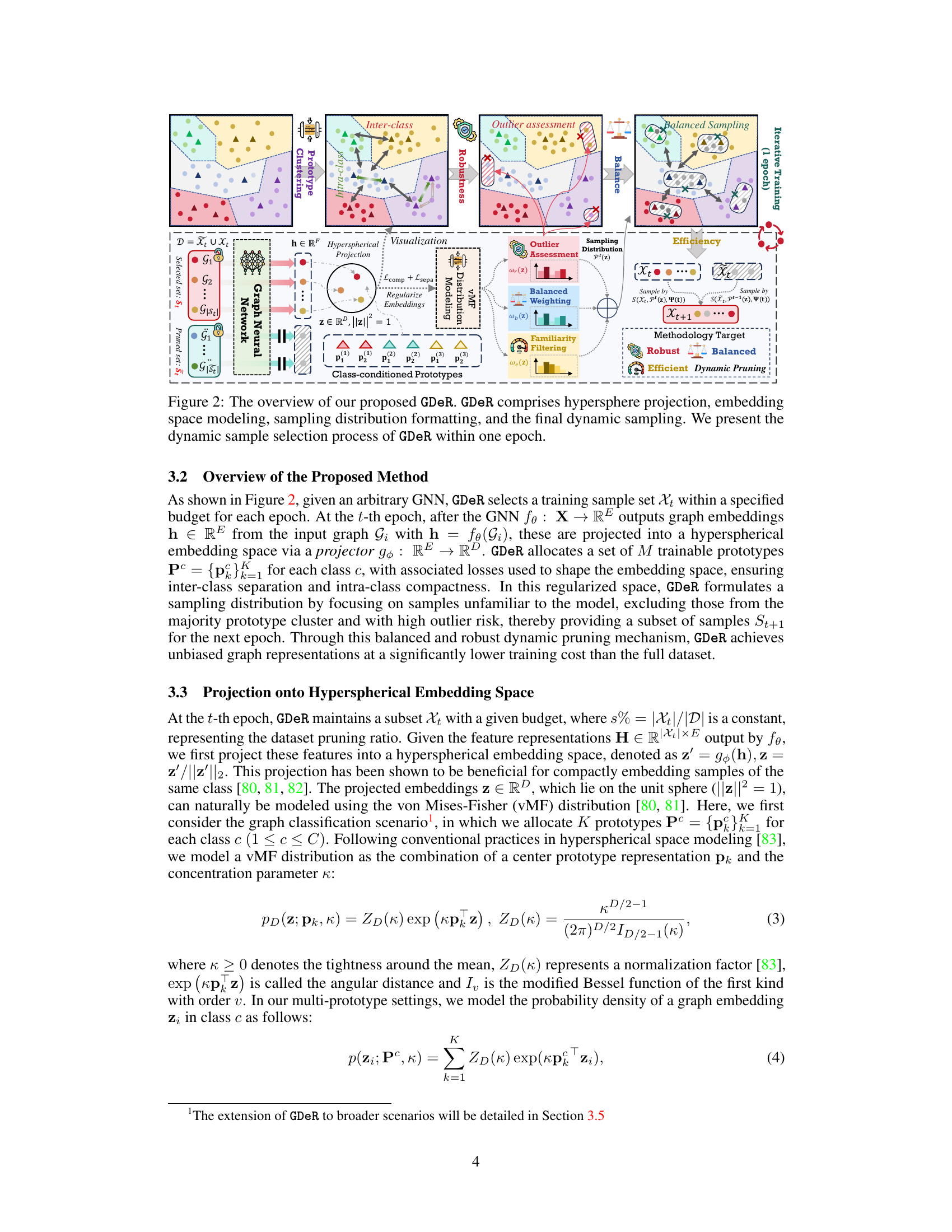
🔼 This figure provides a detailed overview of the proposed GDeR method. It’s a dynamic soft-pruning method designed for efficient and robust graph training. The figure breaks down the GDeR process into four stages: 1. Hyperspherical Projection: Graph samples are projected onto a hypersphere for better embedding space modeling. 2. Embedding Space Modeling: Trainable prototypes are used to shape the embedding space, ensuring inter-class separation and intra-class compactness. 3. Sampling Distribution Formatting: A sampling distribution is created based on outlier risk, model familiarity, and class balance, prioritizing samples that are representative, robust, and unbiased. 4. Dynamic Sampling: The method dynamically selects training samples during the training process based on the sampling distribution. This dynamic selection ensures that both efficiency (by pruning unnecessary samples) and robustness (by handling imbalance and noise) are achieved. The figure visualizes each step and how the process iterates across epochs.
read the caption
Figure 2: The overview of our proposed GDeR. GDeR comprises hypersphere projection, embedding space modeling, sampling distribution formatting, and the final dynamic sampling. We present the dynamic sample selection process of GDeR within one epoch.

🔼 This figure demonstrates the trade-off between training efficiency and model performance for various data pruning methods on the OGB-MOLHIV dataset. The x-axis represents the percentage of the original training time per epoch achieved by each method, while the y-axis shows the corresponding ROC-AUC score. It highlights how GDeR achieves comparable or superior performance to other methods while significantly reducing training time.
read the caption
Figure 3: The trade-off between per epoch time and ROC-AUC (%) of data pruning methods. Specifically, we report the test performance when pruning methods achieve per epoch times of {90%, 70%, 50%, 40%, 30%} of the full dataset training time. 'Vanilla' denotes the original GNN backbone without any data pruning.

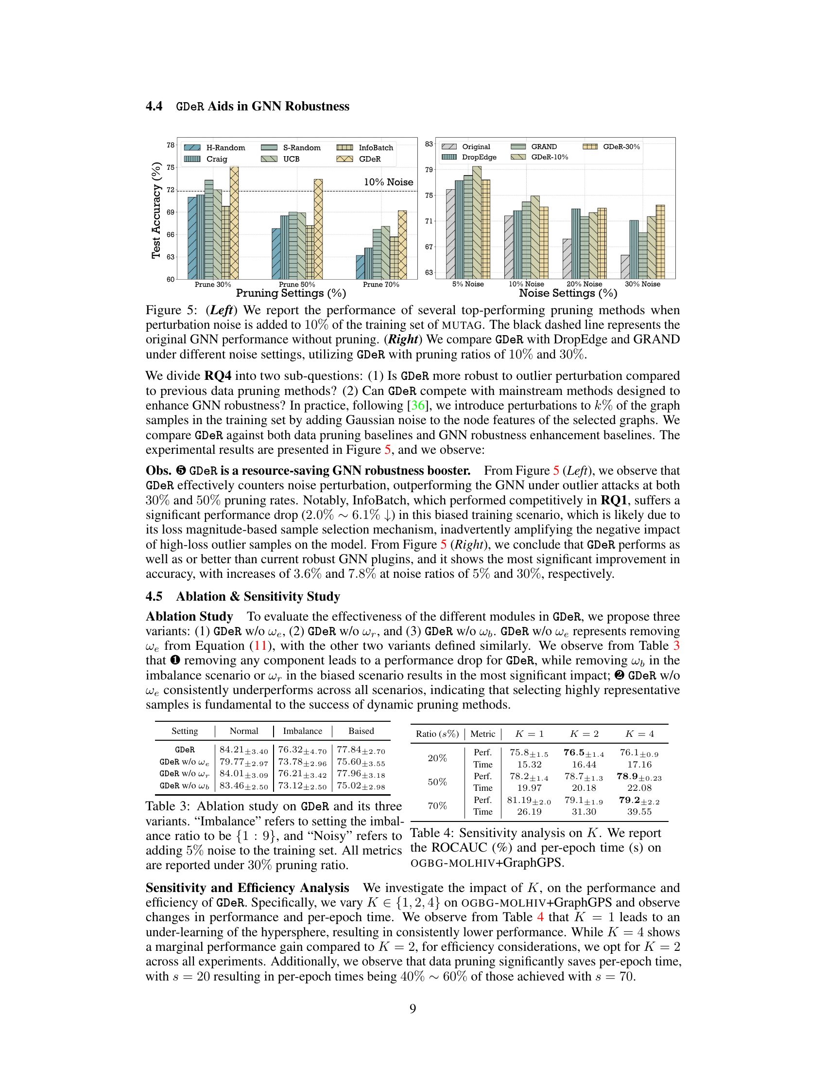
🔼 This figure compares the performance of various data pruning methods, including GDeR, across different imbalance ratios in the MUTAG and DHFR datasets using GCN. The x-axis represents the imbalance ratio (minority:majority), while the y-axis shows the F1-macro score. The ‘No Pruning’ line represents the performance without any pruning. The different lines depict performance with different pruning techniques, highlighting GDeR’s effectiveness in maintaining performance despite significant data imbalance.
read the caption
Figure 4: Performance comparison of different pruning methods across various imbalance ratios. We utilize MUTAG and DHFR datasets with GCN, and reported the metrics when adjusting the imbalance ratios among {1:9, 3:7, 15:57:3, 9:1}. “No Pruning” denotes training GCN without dataset pruning.

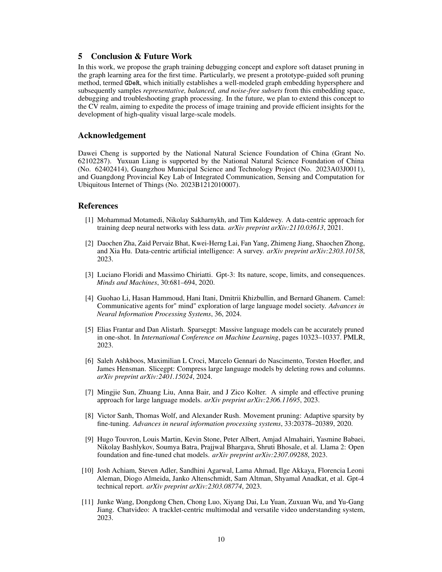
🔼 The left graph shows the test accuracy of different pruning methods on MUTAG dataset with 10% noise added to the training data. The right graph compares the robustness of GDeR against DropEdge and GRAND under different noise levels (5%, 10%, 20%, and 30%).
read the caption
Figure 5: (Left) We report the performance of several top-performing pruning methods when perturbation noise is added to 10% of the training set of MUTAG. The black dashed line represents the original GNN performance without pruning. (Right) We compare GDeR with DropEdge and GRAND under different noise settings, utilizing GDeR with pruning ratios of 10% and 30%.
More on tables
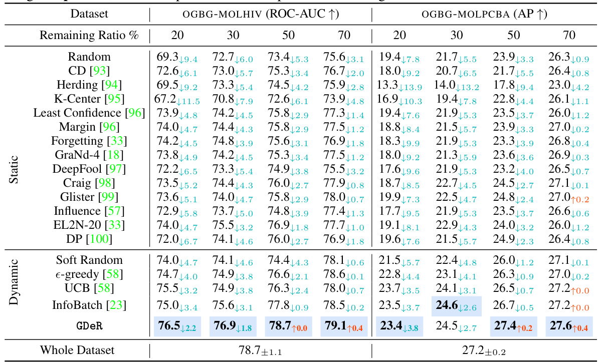
🔼 This table compares the performance of GDeR against 14 static and 3 dynamic data pruning methods across four different remaining ratios (20%, 30%, 50%, 70%) on the OGBG-MOLHIV and OGBG-MOLPCBA datasets. The performance metric used is ROC-AUC for OGBG-MOLHIV and AP for OGBG-MOLPCBA. All methods are trained using the PNA backbone. The results are averages over five runs.
read the caption
Table 1: Performance comparison to state-of-the-art dataset pruning methods when remaining {20%, 30%, 50%, 70%} of the full set. All methods are trained using PNA, and the reported metrics represent the average of five runs.

🔼 This table presents the ablation study results for the proposed GDeR method. It shows the performance of GDeR under normal, imbalanced, and noisy training scenarios when different components (outlier risk assessment, sample familiarity metric, and sample balancing score) are removed. The results demonstrate the contribution of each component to the overall performance of GDeR.
read the caption
Table 3: Ablation study on GDeR and its three variants. 'Imbalance' refers to setting the imbalance ratio to be {1 : 9}, and “Noisy” refers to adding 5% noise to the training set. All metrics are reported under 30% pruning ratio.

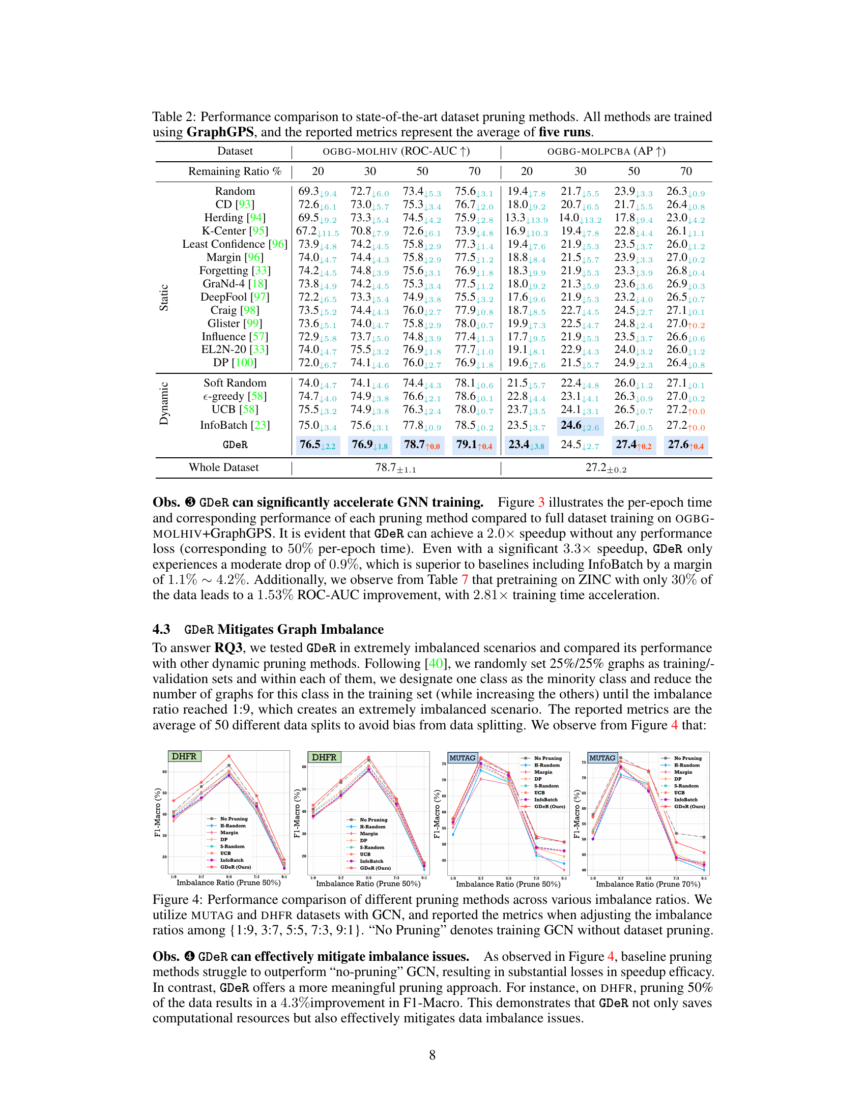
🔼 This table compares the performance of GDeR against other state-of-the-art dataset pruning methods using the GraphGPS model. It shows the ROC-AUC and AP scores for different pruning ratios (20%, 30%, 50%, 70%) across two datasets (OGBG-MOLHIV and OGBG-MOLPCBA). The results highlight GDeR’s performance relative to both static and dynamic pruning methods under various data reduction levels.
read the caption
Table 2: Performance comparison to state-of-the-art dataset pruning methods. All methods are trained using GraphGPS, and the reported metrics represent the average of five runs.

🔼 This table compares the performance of GDeR against other state-of-the-art dataset pruning methods on two datasets (OGBG-MOLHIV and OGBG-MOLPCBA) using the PNA backbone. The table shows the performance (ROC-AUC for OGBG-MOLHIV and Average Precision for OGBG-MOLPCBA) achieved by each method when only a subset of the original data (20%, 30%, 50%, or 70%) is used for training. The results highlight GDeR’s performance relative to other methods, both static and dynamic.
read the caption
Table 1: Performance comparison to state-of-the-art dataset pruning methods when remaining {20%, 30%, 50%, 70%} of the full set. All methods are trained using PNA, and the reported metrics represent the average of five runs.

🔼 This table compares the performance of GDeR against other state-of-the-art dataset pruning methods across four different pruning ratios (20%, 30%, 50%, and 70%). The performance is measured using metrics appropriate for each dataset (ROC-AUC and AP for OGBG datasets, Accuracy and F1-macro for MUTAG and DHFR). The results showcase GDeR’s effectiveness in maintaining or improving performance even with significant data reduction.
read the caption
Table 1: Performance comparison to state-of-the-art dataset pruning methods when remaining {20%, 30%, 50%, 70%} of the full set. All methods are trained using PNA, and the reported metrics represent the average of five runs.

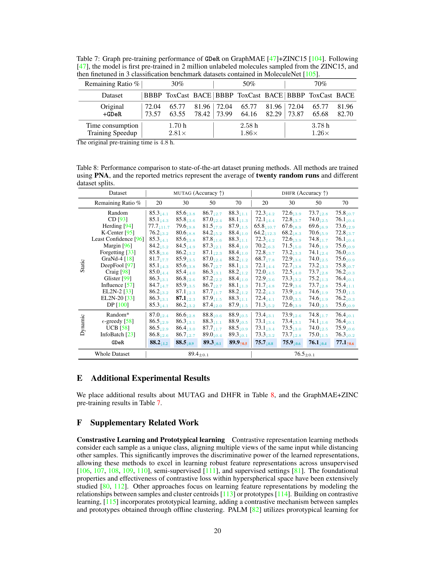
🔼 This table shows the performance of GDeR on the GraphMAE model pre-trained with ZINC15 dataset. It presents the results of three benchmark datasets (BBBP, ToxCast, BACE) with different remaining ratios of the data (30%, 50%, 70%). For each dataset and remaining ratio, the original performance and the performance after applying GDeR are shown, along with the training time and speedup achieved by GDeR. The table demonstrates that GDeR is capable of achieving higher accuracy or comparable accuracy while significantly reducing training time compared to the original training without pruning.
read the caption
Table 7: Graph pre-training performance of GDeR on GraphMAE [47]+ZINC15 [104]. Following [47], the model is first pre-trained in 2 million unlabeled molecules sampled from the ZINC15, and then finetuned in 3 classification benchmark datasets contained in MoleculeNet [105].

🔼 This table presents a comparison of GDeR’s performance against other state-of-the-art static and dynamic dataset pruning methods. The comparison uses the PNA architecture and evaluates performance across four different remaining ratios of the full dataset (20%, 30%, 50%, and 70%). Reported metrics are averages across five independent runs. The table allows assessment of GDeR’s efficiency and performance relative to existing techniques.
read the caption
Table 1: Performance comparison to state-of-the-art dataset pruning methods when remaining {20%, 30%, 50%, 70%} of the full set. All methods are trained using PNA, and the reported metrics represent the average of five runs.
Full paper#
