Abrupt Learning in Transformers: A Case Study on Matrix Completion

O9RZAEp34l

Pulkit Gopalani et el.

TL;DR
#

Large language models (LLMs) are powerful but their learning process remains mysterious. This paper studies a phenomenon known as ‘abrupt learning’ where the training loss plateaus then sharply decreases. To study this in detail, the researchers used a simplified version of the problem: matrix completion, and trained a BERT model on it. This allowed them to understand what happens inside the model.

The study reveals that before the sharp loss drop, the model does little more than copy the existing data. After the drop, however, the model undergoes an ‘algorithmic transition’. It now uses its attention mechanisms to identify and combine relevant parts of the input in a way that lets it accurately fill in the missing values. Attention maps reveal a transition from random patterns to interpretable patterns focused on relevant parts of the input. The paper’s findings deepen our understanding of how LLMs learn and solve tasks.

Key Takeaways
#

Why does it matter?
#

This paper is crucial for researchers studying the training dynamics of large language models (LLMs). It identifies and explains the phenomenon of abrupt learning, a sudden and sharp drop in loss during training, which is a poorly understood yet significant aspect of LLM behavior. This research offers valuable insights into the internal mechanisms of LLMs, contributing to the broader goal of making these models more interpretable and controllable, especially relevant for AI safety and regulation. The findings open avenues for future research to develop more predictable and efficient LLM training methods.

Visual Insights
#

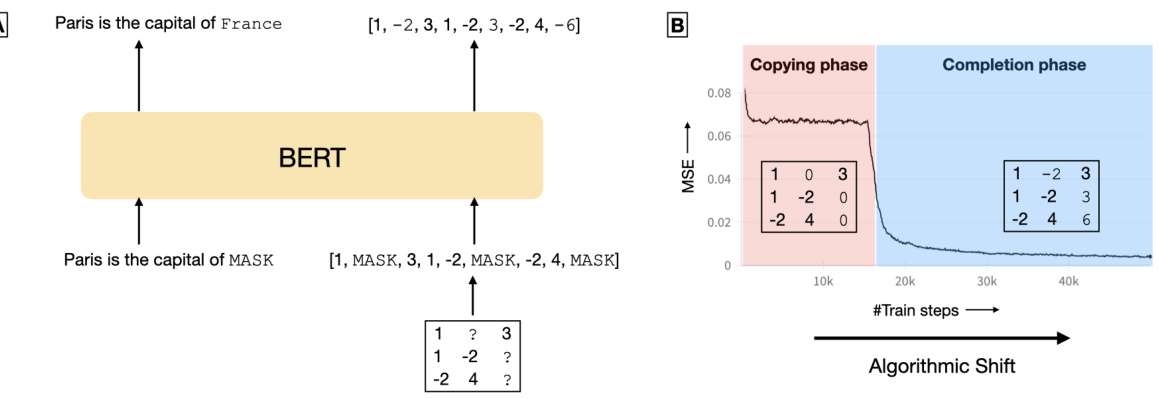
🔼 This figure demonstrates the process of matrix completion using BERT. Panel (A) shows an analogy between masked language modeling and matrix completion tasks. A sentence with masked words is analogous to a matrix with missing entries. Both problems involve using the surrounding context (observed words/matrix entries) to predict the missing elements (masked words/missing entries). Panel (B) displays the training loss curve of a BERT model during matrix completion. The curve showcases a noticeable plateau followed by a sharp decrease in the Mean Squared Error (MSE) loss, revealing an ‘algorithmic shift’ within the model’s approach to the problem. Initially, the model simply copies the input values (copying phase), but after the sudden drop, it transitions into an accurate prediction of the missing entries (completion phase).
read the caption
Figure 1: (A) Matrix completion using BERT. Similar to completing missing words in an English sentence in MLM, we complete missing entries in a masked low-rank matrix. (B) Sudden drop in loss. During training, the model undergoes an algorithmic shift marked by a sharp decrease in mean-squared-error (MSE) loss. Here, the model shifts from simply copying the input (copying phase) to computing missing entries accurately (completion phase).

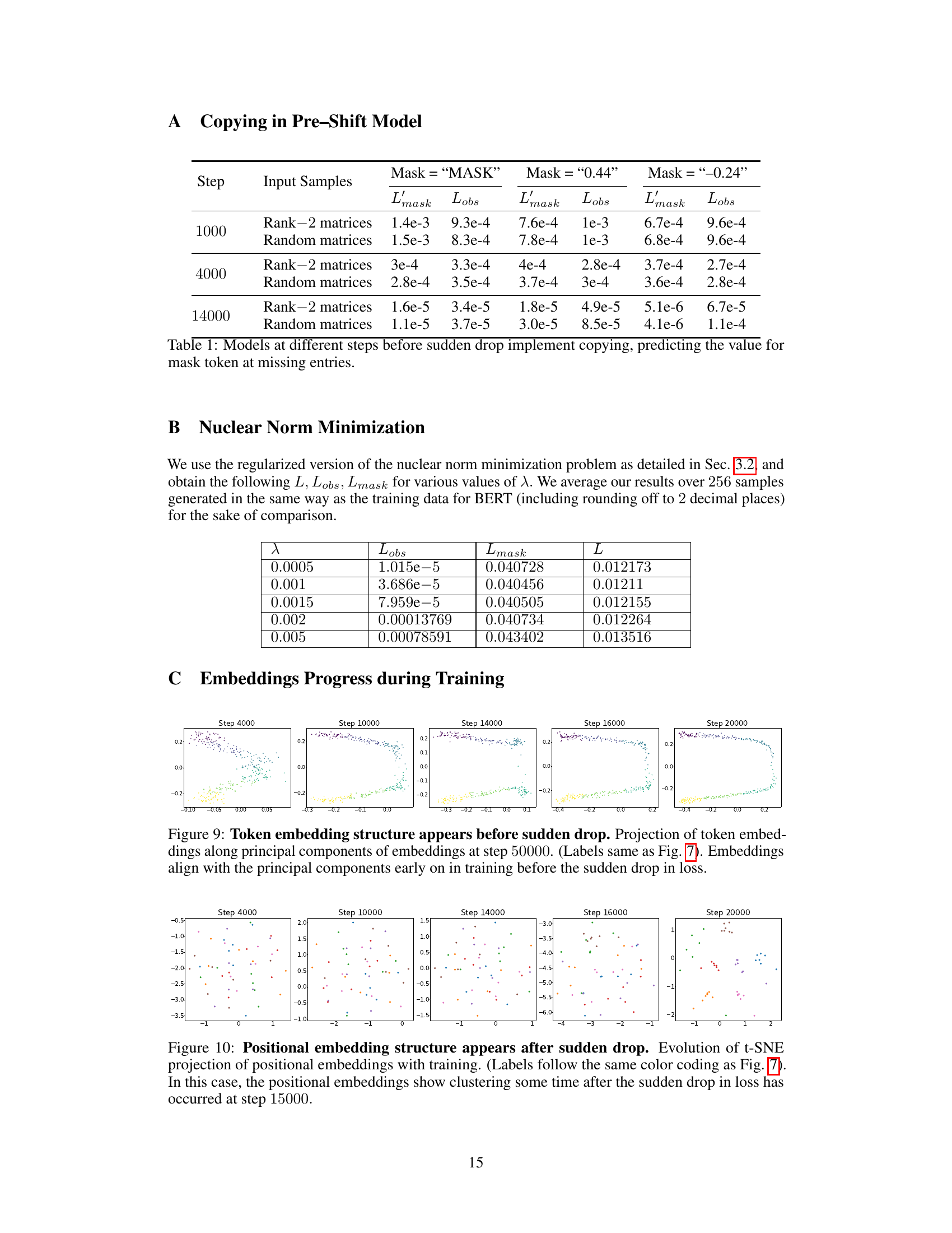
🔼 This table presents the results of an experiment designed to verify that a pre-shift model copies the input values. The experiment involved replacing the masked elements in a 7x7 rank-2 input matrix with various values (MASK, 0.44, -0.24), then measuring the mean squared error (MSE) at both observed and masked positions. The results show that the model outputs values close to the input values at masked positions, indicating a copying behavior rather than accurate prediction of missing entries. The experiment was repeated at different training steps (1000, 4000, 14000) to observe how this behavior changes over time.
read the caption
Table 1: Models at different steps before sudden drop implement copying, predicting the value for mask token at missing entries.

In-depth insights
#

Abrupt Learning
#

The phenomenon of “abrupt learning” in deep neural networks, particularly transformer models, is characterized by prolonged periods of minimal training progress followed by a sudden and dramatic improvement in performance. This unexpected shift challenges our understanding of the learning process, defying traditional models of gradual optimization. The paper investigates this abrupt change using matrix completion as a simplified model. It reveals that this abrupt transition is not merely a change in loss, but reflects a fundamental shift in the model’s underlying algorithm. Initially, the model uses a simpler approach (copying), then suddenly transitions to a more complex and efficient algorithm for solving the task. Interpretability analyses show this transition involves a change in attention mechanisms and the encoding of relevant information in hidden states. The timing of the changes in different model components (embeddings, attention layers, MLPs) suggests a cascade effect, where learning in certain parts triggers improvements in others. This “abrupt learning” behavior raises important questions about the dynamics of deep learning and the need for more sophisticated models of learning processes. Further research should focus on generalizing these findings to more complex tasks and architectures, to fully understand this intriguing phenomenon and to improve the design and training of deep learning models.

BERT Matrix
#

A hypothetical “BERT Matrix” section in a research paper would likely explore using BERT, a transformer-based language model, for matrix-related tasks. This could involve several approaches. One might focus on representing matrices as text sequences, allowing BERT to learn patterns and relationships between matrix elements through its contextual understanding. Another approach could leverage BERT’s attention mechanism to identify relevant parts of a matrix for specific operations, such as prediction or completion of missing values. The core idea would likely be to exploit BERT’s ability to learn complex relationships from data to perform matrix-related operations that are normally addressed by numerical methods. The section would likely detail the specific tasks tackled (e.g., matrix completion, prediction), the methodology for converting matrices into BERT-compatible input, and the evaluation metrics used to measure performance. A key aspect would be comparing BERT’s performance against traditional algorithms. Success would demonstrate the potential of applying deep learning techniques to solve matrix problems traditionally solved by linear algebra. Further, the research might also investigate the interpretability of BERT’s approach to gain insights into how the model represents and reasons about matrices, potentially leading to new insights in both matrix computations and neural network interpretability. The findings could have implications for improving efficiency, robustness or generalization abilities of matrix-solving algorithms. Therefore, a comprehensive evaluation would be crucial to establishing the viability and advantages of this novel approach.

Algorithmic Shift
#

The concept of “Algorithmic Shift” in the context of transformer model training, as discussed in the paper, points to a critical transition in the model’s behavior during the learning process. Initially, the model adopts a simple, less efficient strategy, such as copying input values for missing entries in a matrix completion task. However, at a certain point, marked by a sharp drop in the training loss, the model undergoes an abrupt change, transitioning to a more sophisticated and accurate approach. This shift represents a fundamental change in the algorithm implicitly employed by the model. It’s not a gradual improvement, but rather a distinct qualitative change in how the model solves the problem. This transition is accompanied by observable changes in attention mechanisms and internal representations, indicating a reorganization of the model’s internal structure and its capacity to process information. The paper suggests that this ‘algorithmic shift’ might be a general phenomenon in large language models, representing a key aspect of their learning dynamics.

Model Dynamics
#

Analyzing model dynamics offers crucial insights into the learning process of complex models. Understanding how different components of a model evolve over time is key to interpreting the overall performance and identifying potential bottlenecks. For example, investigating the training dynamics of attention heads reveals when and how they learn to focus on relevant information. Tracking the changes in embeddings helps us assess how well the model represents the input data and its evolution. Similarly, examining the dynamics of MLP layers reveals how the non-linear transformations contribute to the model’s predictive capacity. By carefully analyzing these individual components, we gain a more comprehensive understanding of the model’s learning trajectory, pinpoint crucial phases such as algorithmic shifts or phase transitions, and gain valuable insight into potential improvements or optimizations. These insights can lead to a deeper understanding of the learning mechanisms and improvements in training strategies and model architectures.

Future Work
#

Future research directions stemming from this work could explore several promising avenues. Extending the matrix completion experiments to larger matrices and higher ranks is crucial to assess the scalability and generalizability of the observed abrupt learning phenomenon. A deeper investigation into the algorithmic transition’s precise mechanism is needed, possibly involving techniques from mechanistic interpretability to unravel the model’s internal computations during this phase transition. Exploring different architectures beyond BERT (e.g., transformers with different attention mechanisms or other neural network types) would further illuminate the generality of abrupt learning. Finally, it would be valuable to investigate the role of various hyperparameters and training settings on the abrupt learning, systematically varying parameters like learning rate, batch size, and optimizer to see if these influence the occurrence or timing of the transition. Further research should also analyze the performance across diverse matrix completion tasks, potentially comparing against other established algorithms like nuclear norm minimization.

More visual insights
#

More on figures

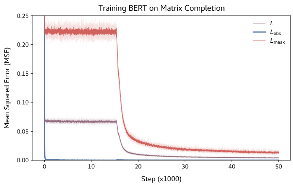
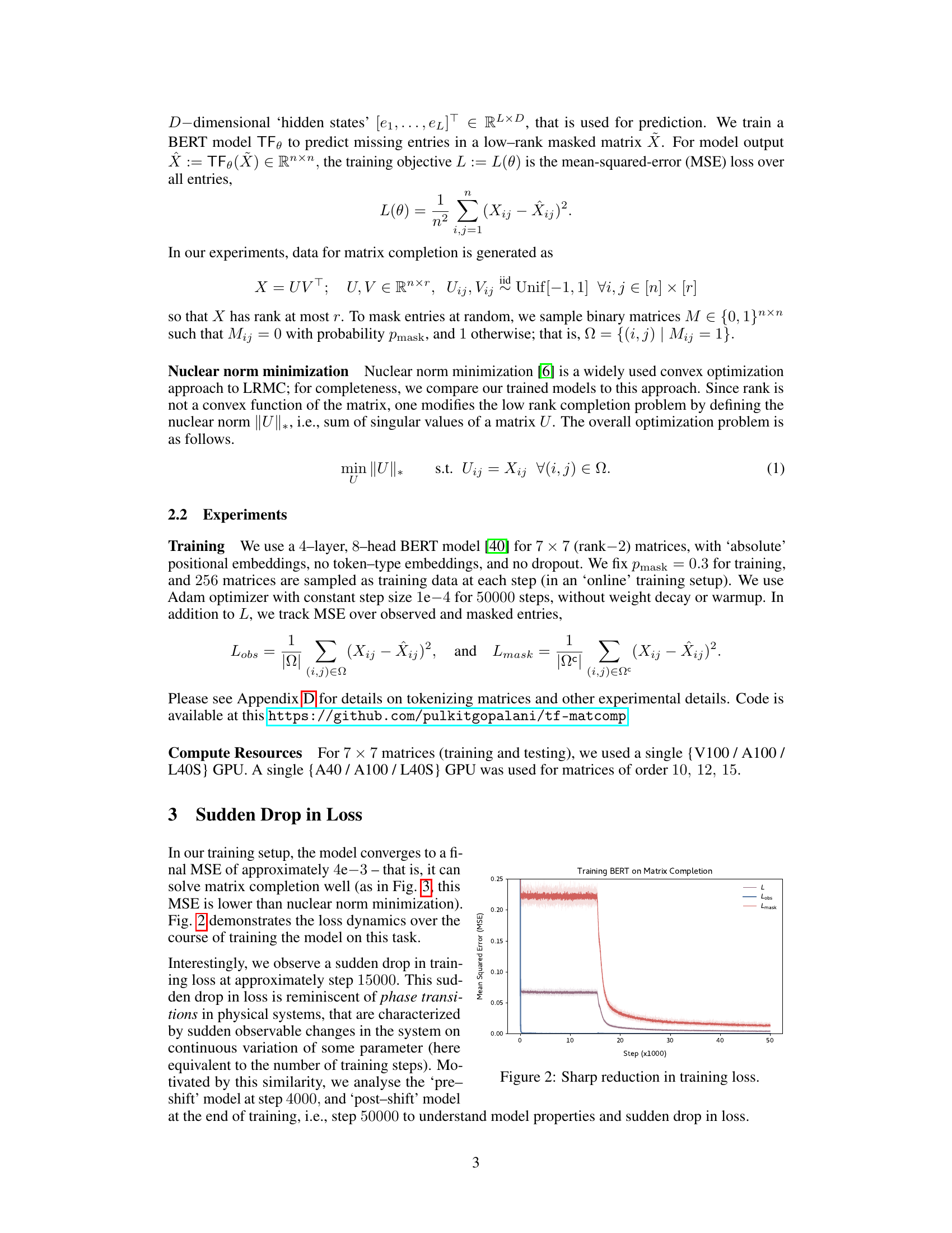
🔼 This figure shows the training loss curves for the BERT model trained on the matrix completion task. The plot shows three different loss curves: the total loss (L), the loss on observed entries (Lobs), and the loss on masked entries (Lmask). It highlights the sudden drop in loss that occurs after an initial plateau, indicating a shift in the model’s learning algorithm.
read the caption
Figure 2: Sharp reduction in training loss.

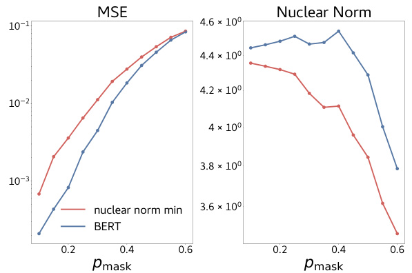
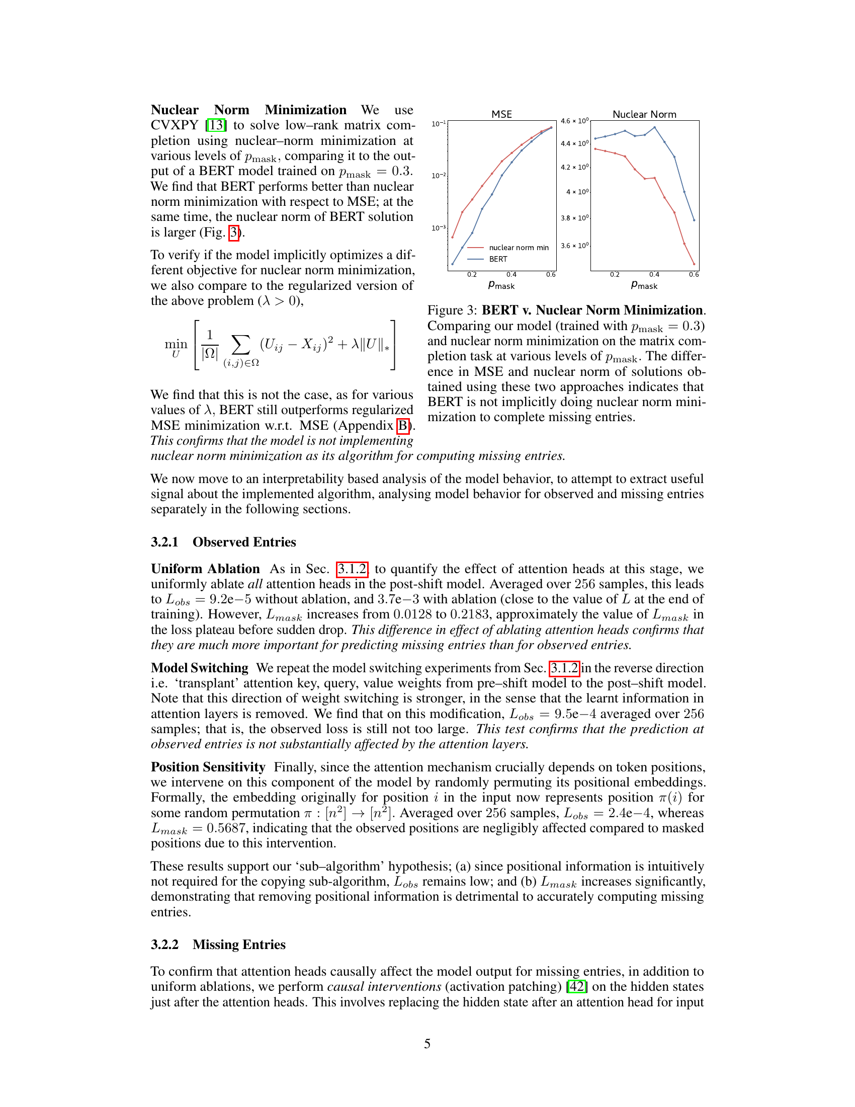
🔼 This figure compares the performance of the BERT model and the nuclear norm minimization algorithm on the matrix completion task. The x-axis represents different masking probabilities ( ), and the y-axis shows the Mean Squared Error (MSE) loss and the nuclear norm of the solution. The results show that the BERT model achieves lower MSE than the nuclear norm minimization, suggesting it doesn’t simply implement this algorithm. The difference in the nuclear norm of the solution further strengthens this point.
read the caption
Figure 3: BERT v. Nuclear Norm Minimization. Comparing our model (trained with = 0.3) and nuclear norm minimization on the matrix completion task at various levels of . The difference in MSE and nuclear norm of solutions obtained using these two approaches indicates that BERT is not implicitly doing nuclear norm minimization to complete missing entries.

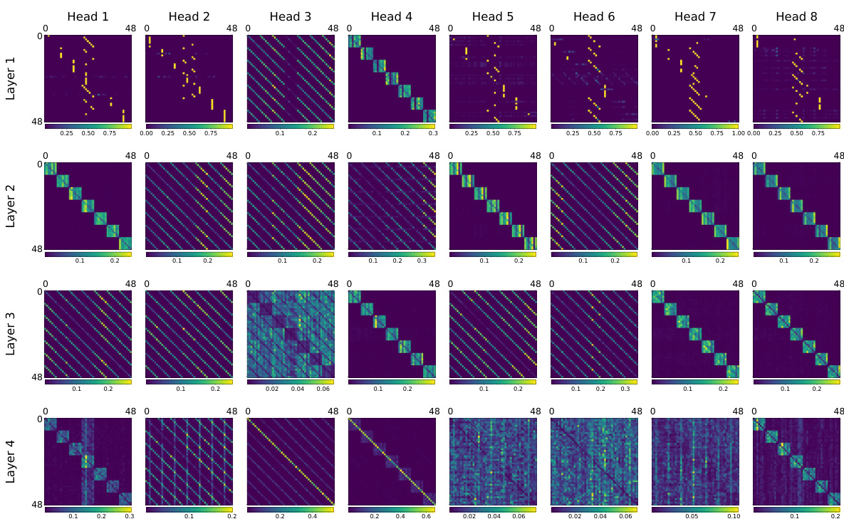
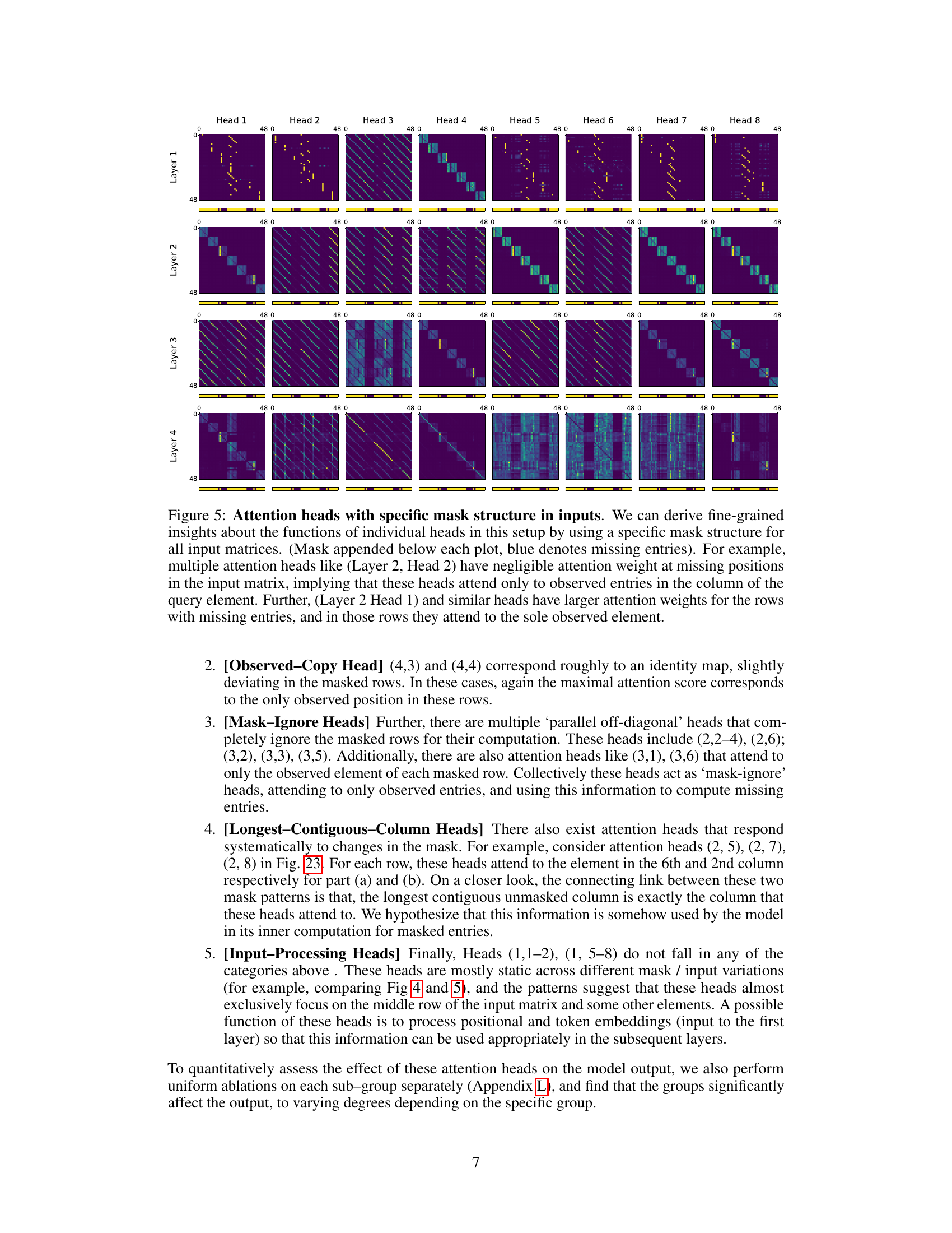
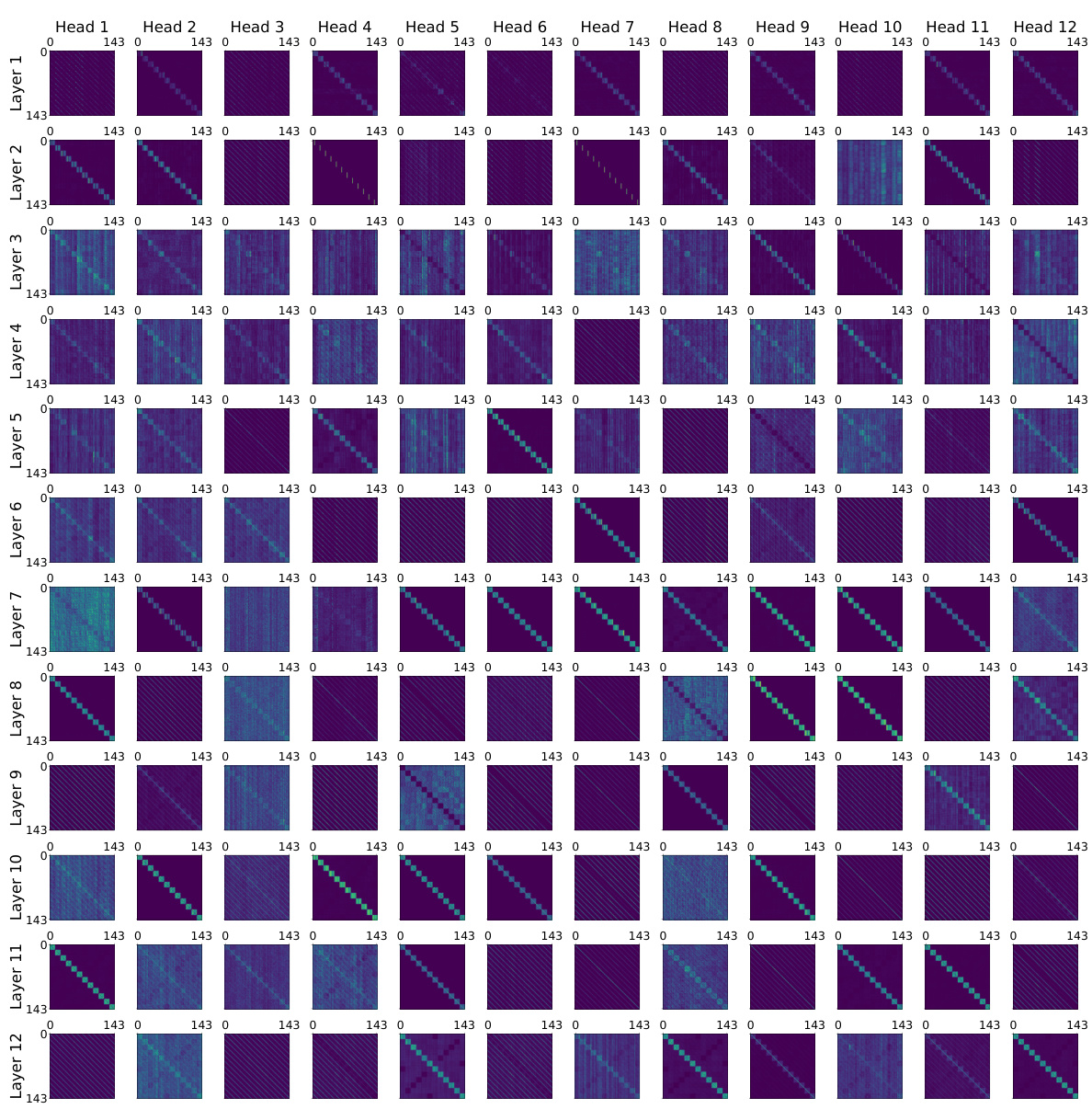
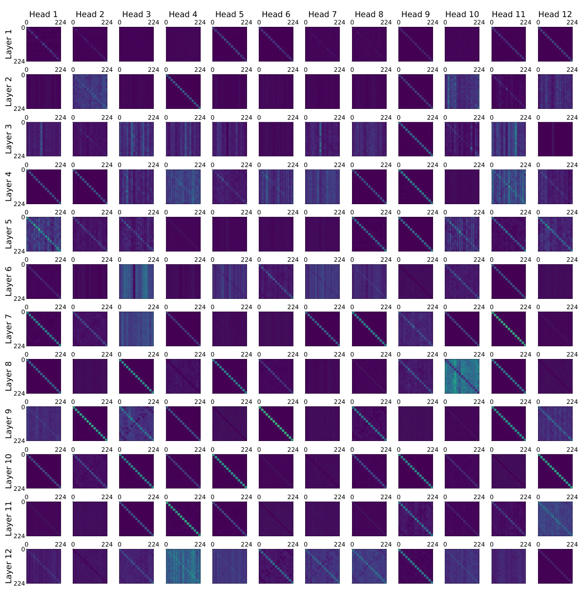
🔼 This figure shows the attention heads of a BERT model at different training steps (4000, 14000, 16000, and 20000). Each subplot represents a different head and layer, visualizing the attention weights as a heatmap. The change in attention patterns over time demonstrates the model’s transition from a copying phase to an accurate matrix completion phase, where the attention heads learn to focus on relevant tokens for accurate prediction. The evolution highlights the shift from uninterpretable attention patterns to interpretable structures, relevant to matrix completion.
read the caption
Figure 22: Attention heads across various training steps.

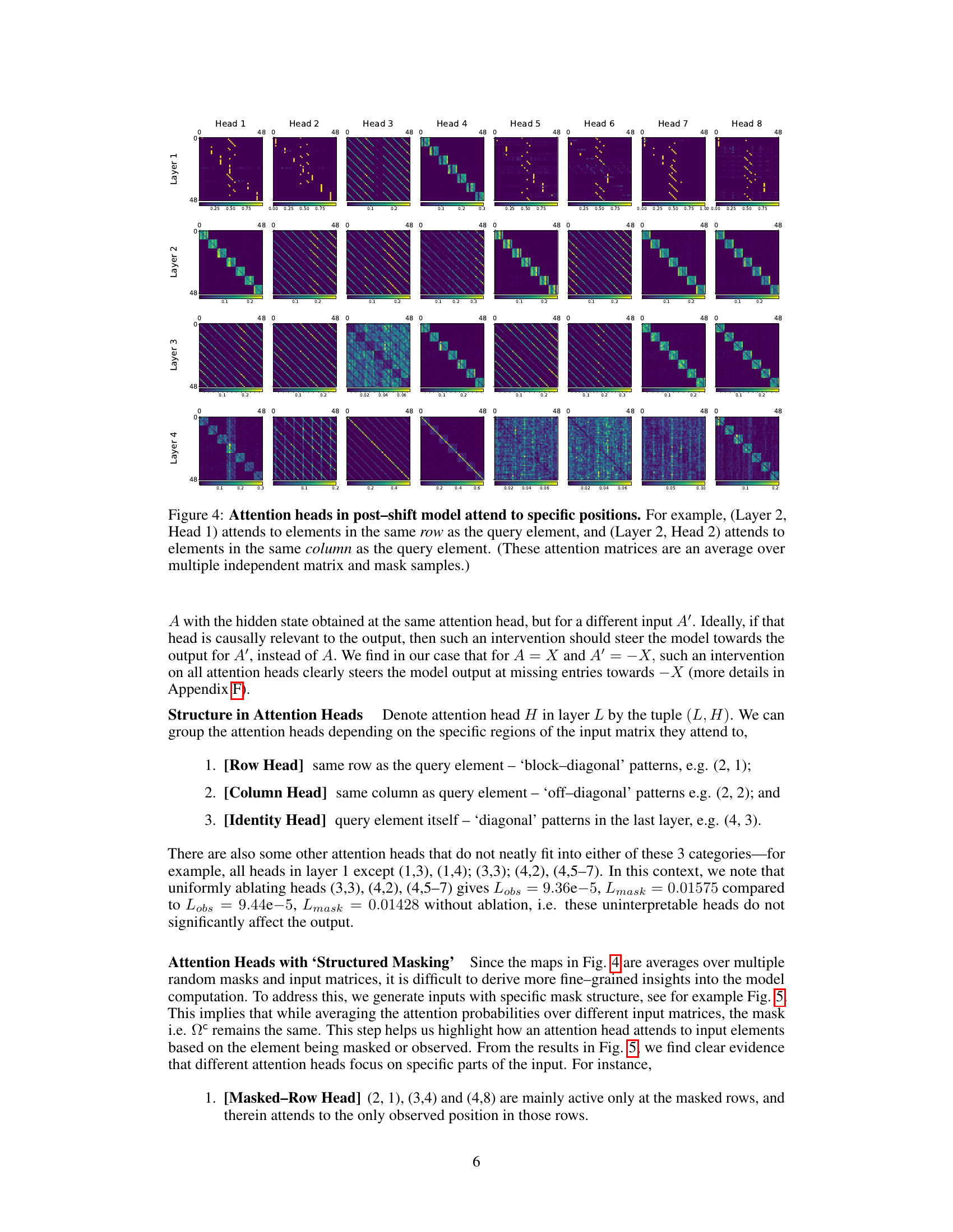
🔼 This figure shows the attention maps of different attention heads in the post-shift model. It demonstrates that after the algorithmic shift, the attention heads develop interpretable patterns relevant to the matrix completion task. Some heads focus on rows, others on columns, indicating a structured approach to identifying and utilizing the relevant contextual information for prediction. The visualization is an average across multiple examples, highlighting consistent attention patterns.
read the caption
Figure 4: Attention heads in post-shift model attend to specific positions. For example, (Layer 2, Head 1) attends to elements in the same row as the query element, and (Layer 2, Head 2) attends to elements in the same column as the query element. (These attention matrices are an average over multiple independent matrix and mask samples.)

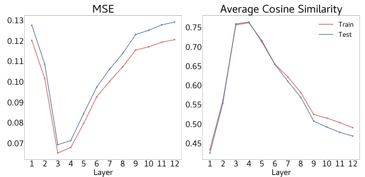
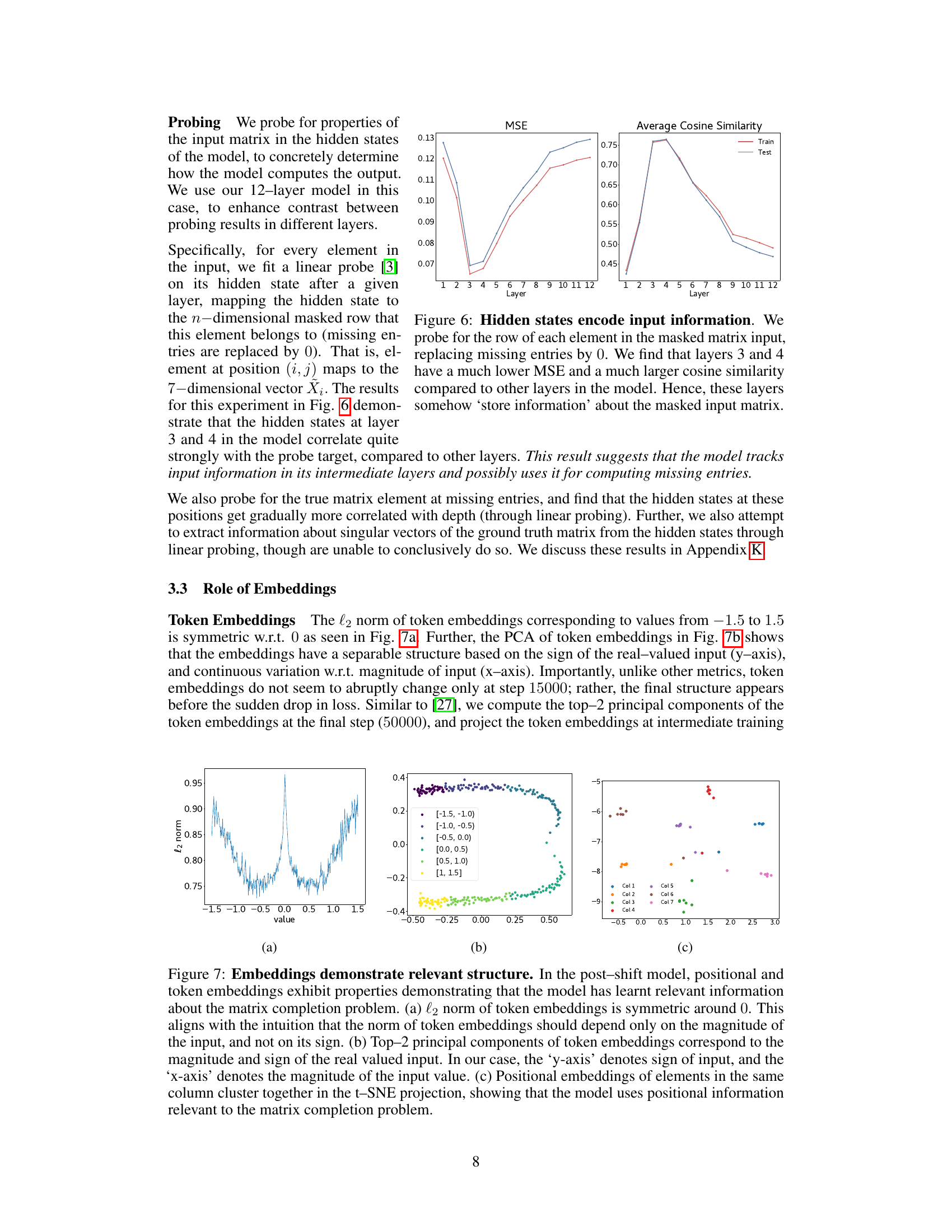
🔼 The figure shows the result of probing the hidden states of the model to check if they encode information about the input matrix. It shows the mean squared error (MSE) and average cosine similarity for each layer of the model when predicting the row of each element. Layers 3 and 4 exhibit significantly lower MSE and higher cosine similarity, indicating that these layers effectively store information about the input matrix.
read the caption
Figure 6: Hidden states encode input information. We probe for the row of each element in the masked matrix input, replacing missing entries by 0. We find that layers 3 and 4 have a much lower MSE and a much larger cosine similarity compared to other layers in the model. Hence, these layers somehow ‘store information’ about the masked input matrix.

🔼 This figure shows three subplots visualizing the properties of token and positional embeddings in the post-shift model. Subplot (a) presents the l2 norm of token embeddings, which is symmetric around 0, indicating dependence only on input magnitude. Subplot (b) displays the top-2 principal components of token embeddings, revealing that they capture input sign and magnitude. Subplot (c) uses t-SNE projection of positional embeddings, showing that embeddings within the same column cluster together, suggesting the model’s use of positional information in solving the matrix completion task.
read the caption
Figure 7: Embeddings demonstrate relevant structure. In the post-shift model, positional and token embeddings exhibit properties demonstrating that the model has learnt relevant information about the matrix completion problem. (a) l2 norm of token embeddings is symmetric around 0. This aligns with the intuition that the norm of token embeddings should depend only on the magnitude of the input, and not on its sign. (b) Top-2 principal components of token embeddings correspond to the magnitude and sign of the real valued input. In our case, the 'y-axis' denotes sign of input, and the 'x-axis' denotes the magnitude of the input value. (c) Positional embeddings of elements in the same column cluster together in the t–SNE projection, showing that the model uses positional information relevant to the matrix completion problem.

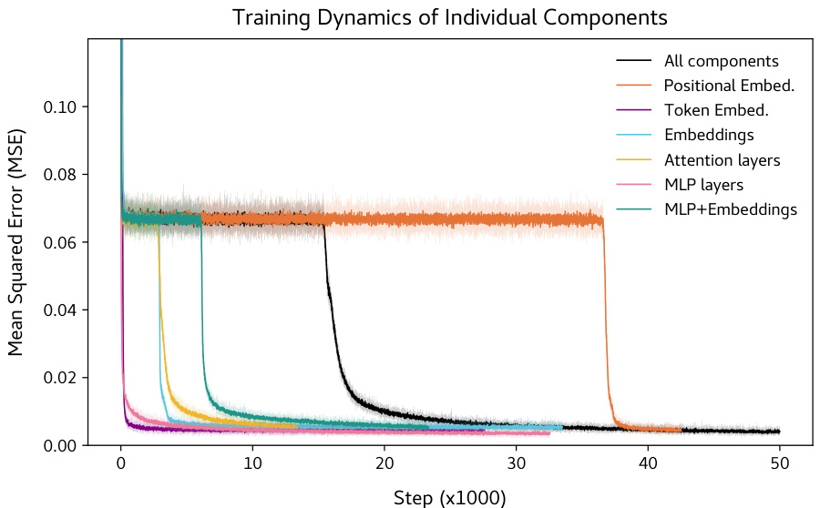
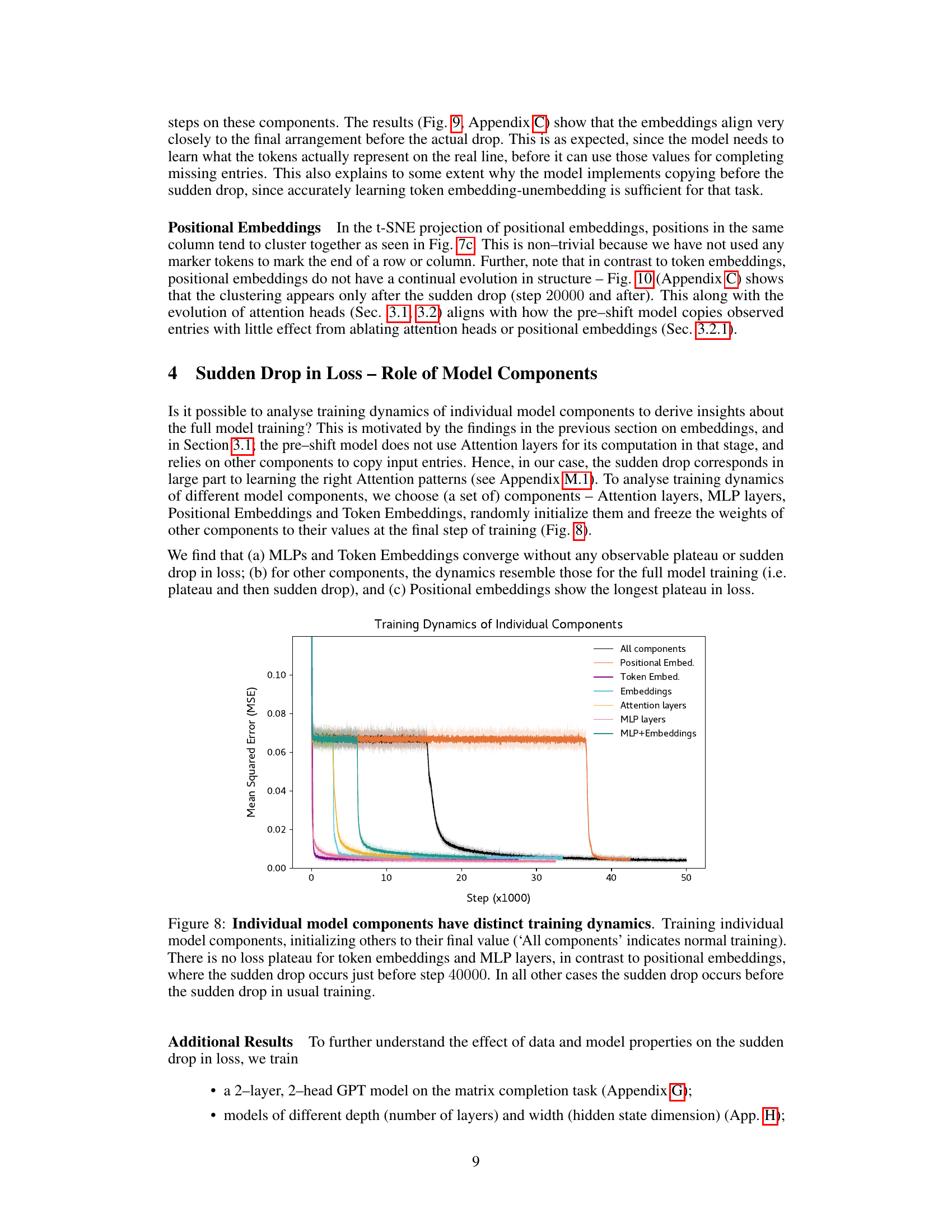
🔼 This figure shows the training dynamics of individual components of the BERT model used for matrix completion. By freezing weights of all components except one, and training only that one component, the authors analyze how each component contributes to the overall training dynamics and the sudden drop in loss. The figure highlights the differences in training behavior between different components, particularly regarding the presence or absence of a plateau before the sharp decrease in loss.
read the caption
Figure 8: Individual model components have distinct training dynamics. Training individual model components, initializing others to their final value (‘All components’ indicates normal training). There is no loss plateau for token embeddings and MLP layers, in contrast to positional embeddings, where the sudden drop occurs just before step 40000. In all other cases the sudden drop occurs before the sudden drop in usual training.

🔼 This figure shows the analysis of token and positional embeddings in the post-shift model. Subfigure (a) demonstrates the symmetry of the l2 norm of token embeddings around 0, indicating that the norm depends only on the magnitude, not the sign of the input. Subfigure (b) uses PCA to reveal that the top two principal components of the embeddings correspond to input magnitude and sign. Subfigure (c) shows the t-SNE projection of positional embeddings, revealing that embeddings in the same column cluster together. This suggests that the model utilizes learned positional information related to the matrix completion task.
read the caption
Figure 7: Embeddings demonstrate relevant structure. In the post-shift model, positional and token embeddings exhibit properties demonstrating that the model has learnt relevant information about the matrix completion problem. (a) l2 norm of token embeddings is symmetric around 0. This aligns with the intuition that the norm of token embeddings should depend only on the magnitude of the input, and not on its sign. (b) Top-2 principal components of token embeddings correspond to the magnitude and sign of the real valued input. In our case, the 'y-axis' denotes sign of input, and the 'x-axis' denotes the magnitude of the input value. (c) Positional embeddings of elements in the same column cluster together in the t–SNE projection, showing that the model uses positional information relevant to the matrix completion problem.

🔼 This figure shows the properties of token and positional embeddings in the post-shift model. The l2 norm of token embeddings is symmetric around 0, indicating the norm depends only on the magnitude of input. PCA of token embeddings shows the top-2 components representing magnitude and sign of the input. The t-SNE projection of positional embeddings shows that elements in the same column cluster together, indicating the model uses positional information relevant to the matrix completion task.
read the caption
Figure 7: Embeddings demonstrate relevant structure. In the post-shift model, positional and token embeddings exhibit properties demonstrating that the model has learnt relevant information about the matrix completion problem. (a) l2 norm of token embeddings is symmetric around 0. This aligns with the intuition that the norm of token embeddings should depend only on the magnitude of the input, and not on its sign. (b) Top-2 principal components of token embeddings correspond to the magnitude and sign of the real valued input. In our case, the 'y-axis' denotes sign of input, and the 'x-axis' denotes the magnitude of the input value. (c) Positional embeddings of elements in the same column cluster together in the t–SNE projection, showing that the model uses positional information relevant to the matrix completion problem.

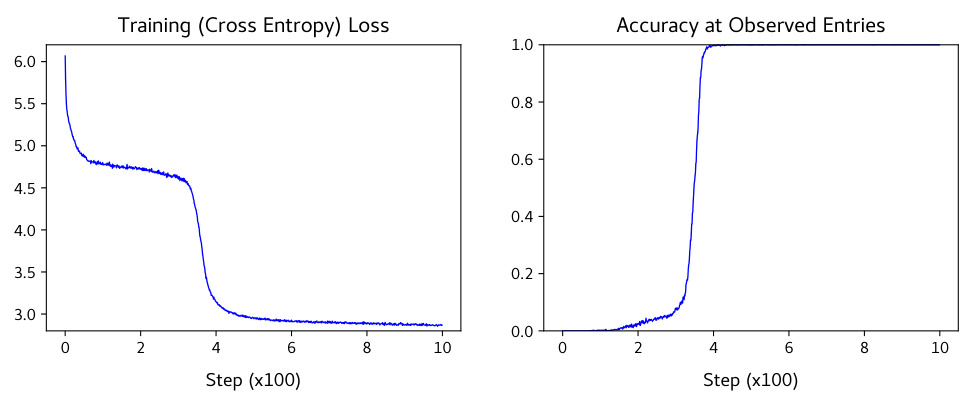
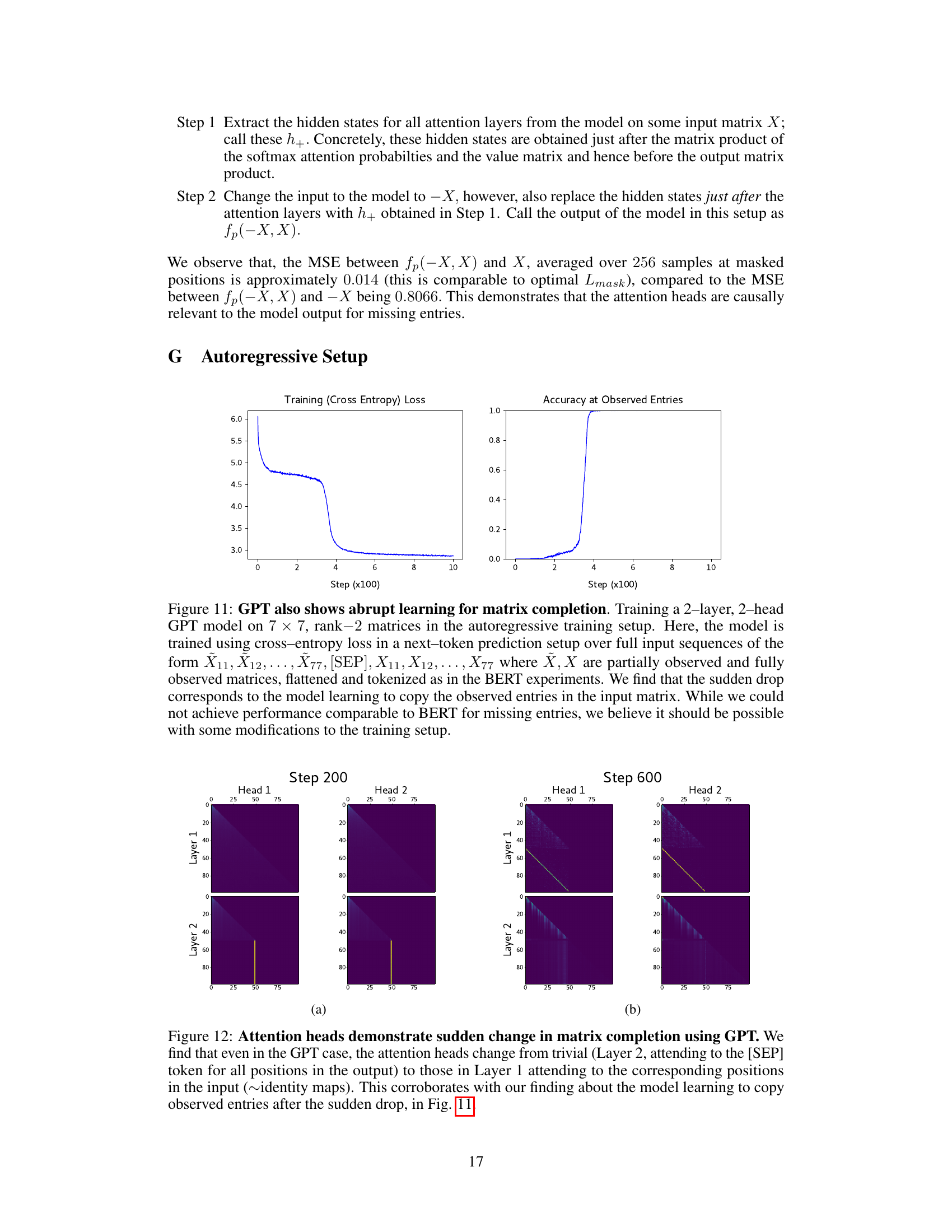
🔼 The figure shows the training loss and accuracy of a 2-layer, 2-head GPT model trained on a matrix completion task using an autoregressive approach. The sudden drop in loss and rapid increase in accuracy at observed entries indicates a similar ‘algorithmic shift’ as observed in the BERT model, characterized by a transition from copying input to accurate prediction.
read the caption
Figure 11: GPT also shows abrupt learning for matrix completion. Training a 2-layer, 2-head GPT model on 7 × 7, rank-2 matrices in the autoregressive training setup. Here, the model is trained using cross-entropy loss in a next–token prediction setup over full input sequences of the form X11, X12, ..., X77, [SEP], X11, X12, ..., X77 where X, X are partially observed and fully observed matrices, flattened and tokenized as in the BERT experiments. We find that the sudden drop corresponds to the model learning to copy the observed entries in the input matrix. While we could not achieve performance comparable to BERT for missing entries, we believe it should be possible with some modifications to the training setup.

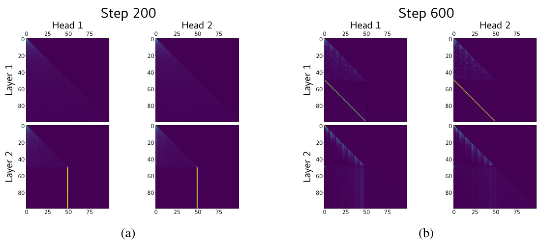
🔼 This figure shows the attention heads of a GPT model during matrix completion at different training steps. In the early stage (Step 200), the attention patterns are largely uniform, indicating that the model does not focus on specific parts of the input. However, as training progresses (Step 600), the attention heads develop clear, interpretable patterns, showing that the model learns to attend to relevant positions in the input matrix corresponding to the output position. This transition is consistent with the model shifting from simply copying the observed entries to actively computing missing entries.
read the caption
Figure 12: Attention heads demonstrate sudden change in matrix completion using GPT. We find that even in the GPT case, the attention heads change from trivial (Layer 2, attending to the [SEP] token for all positions in the output) to those in Layer 1 attending to the corresponding positions in the input (~identity maps). This corroborates with our finding about the model learning to copy observed entries after the sudden drop, in Fig. 11.

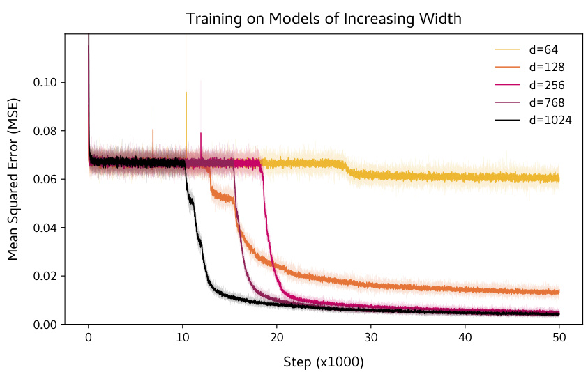
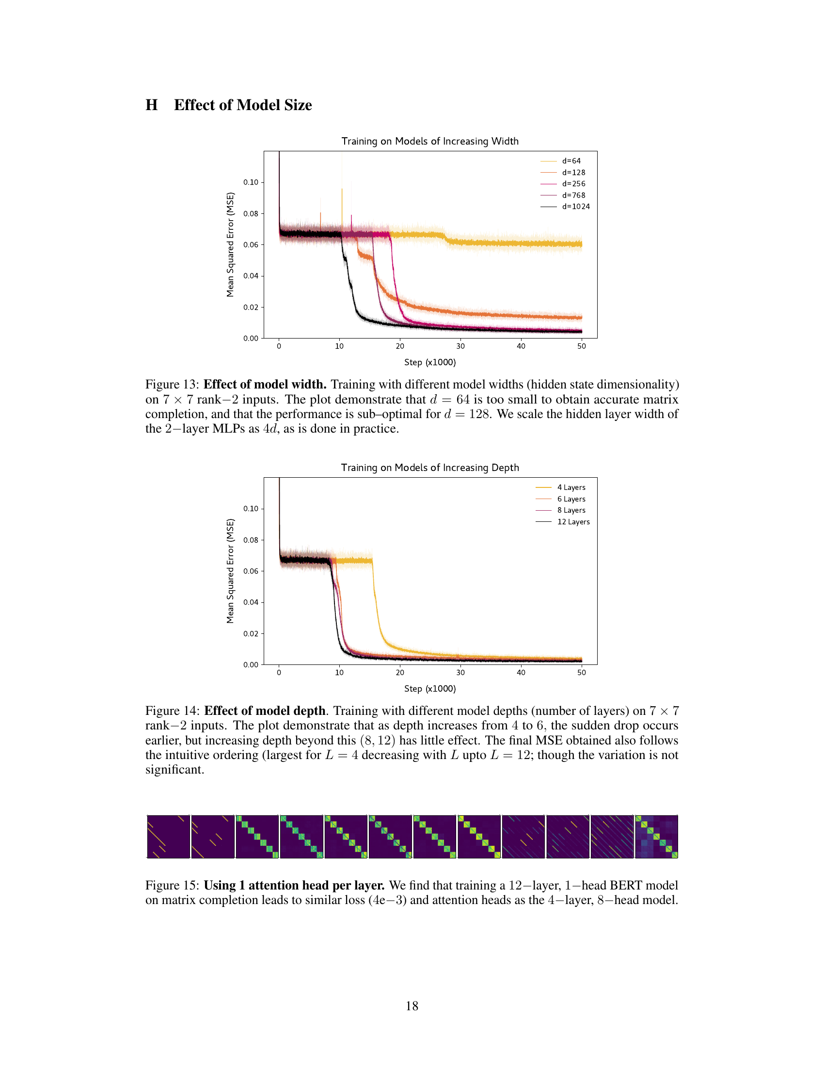
🔼 This figure shows the effect of varying the hidden state dimensionality (model width) on the performance of a BERT model trained for matrix completion. It demonstrates a performance improvement as model width increases from 64 to 1024, indicating that larger models are better suited for this task. However, even with the largest width tested (1024), the model does not perfectly solve the problem.
read the caption
Figure 13: Effect of model width. Training with different model widths (hidden state dimensionality) on 7 × 7 rank-2 inputs. The plot demonstrate that d = 64 is too small to obtain accurate matrix completion, and that the performance is sub-optimal for d = 128. We scale the hidden layer width of the 2-layer MLPs as 4d, as is done in practice.

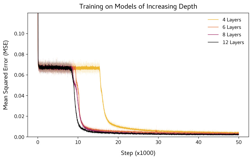
🔼 This figure shows the training loss curves for BERT models with varying depths (number of layers) trained on a 7x7 rank-2 matrix completion task. It demonstrates that increasing the depth from 4 to 6 layers causes the sudden drop in training loss to happen earlier. However, further increasing the depth beyond 6 layers (to 8 or 12) does not significantly affect the timing or magnitude of the sudden drop. The final mean squared error (MSE) also shows a trend of decreasing with increasing depth, although the difference isn’t substantial.
read the caption
Figure 14: Effect of model depth. Training with different model depths (number of layers) on 7 × 7 rank-2 inputs. The plot demonstrate that as depth increases from 4 to 6, the sudden drop occurs earlier, but increasing depth beyond this (8, 12) has little effect. The final MSE obtained also follows the intuitive ordering (largest for L = 4 decreasing with L upto L = 12; though the variation is not significant.

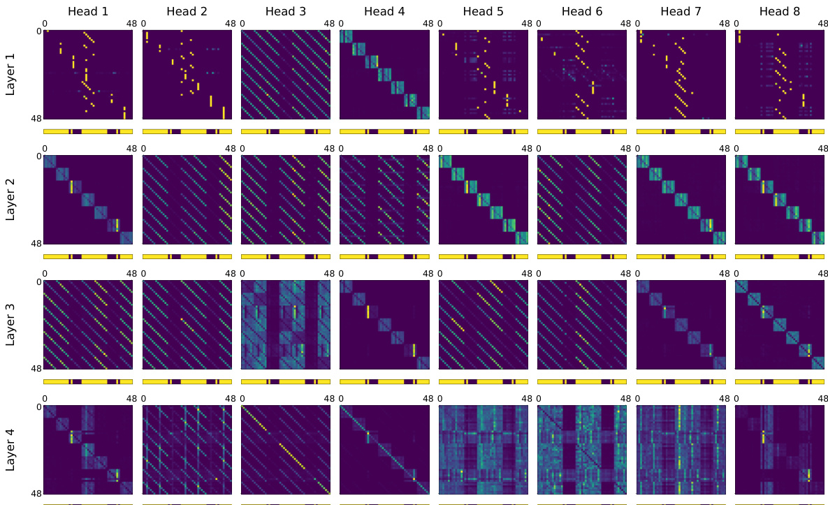
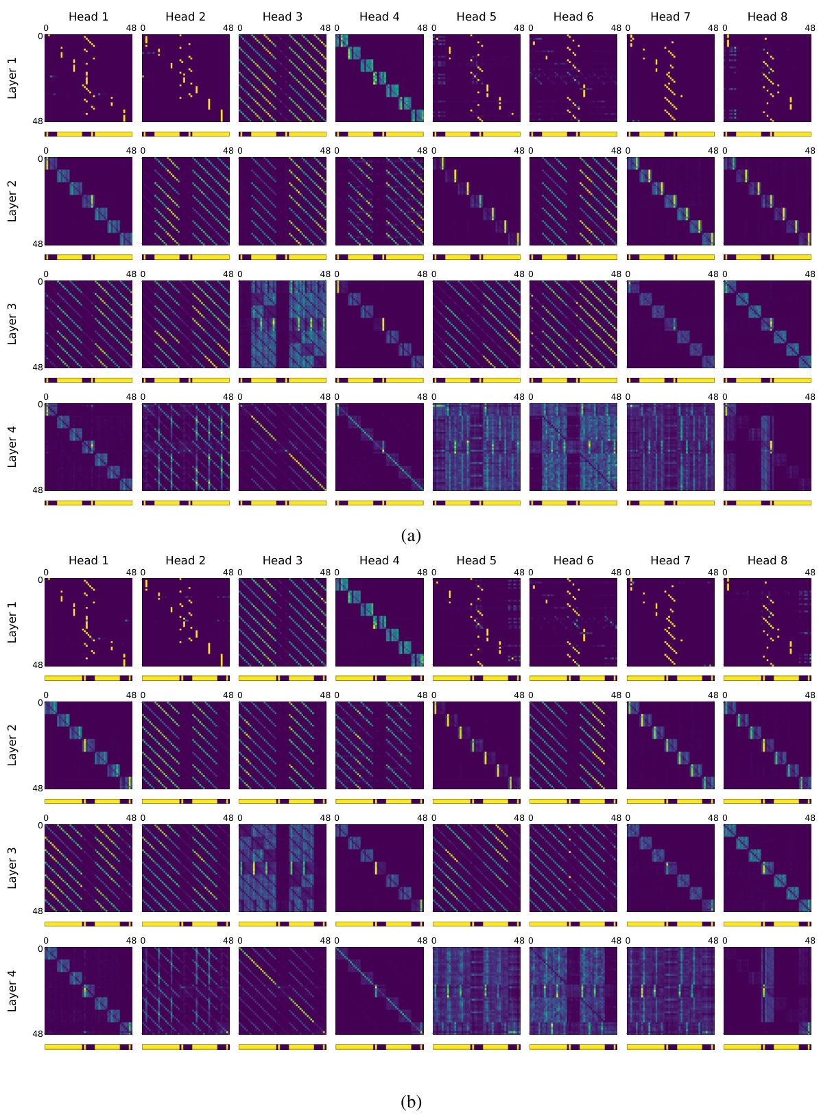
🔼 This figure shows the attention maps of different heads at various layers of the BERT model trained for matrix completion task, along with the corresponding mask patterns used during training. The color intensity in each cell represents the attention weight, and blue color denotes that the entry was masked out in the input matrix. The figure demonstrates that different attention heads focus on different parts of the input matrix. Some heads primarily attend to observed entries within the same row or column as the query element. Others focus on longer contiguous unmasked columns or attend to observed elements in specific rows while completely ignoring others. This variety in the attention patterns highlights the complexity of the model’s internal mechanisms during matrix completion.
read the caption
Figure 23: Attention heads and corresponding masks; blue denotes masked position in the input matrix.

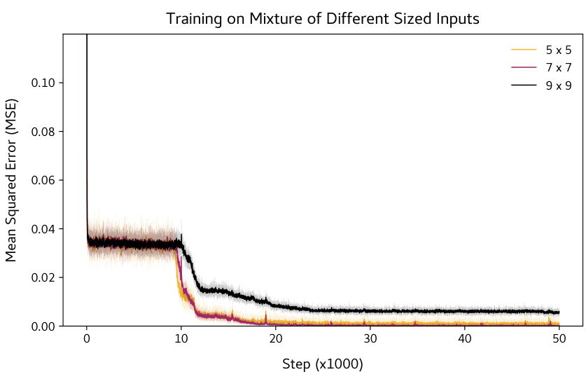
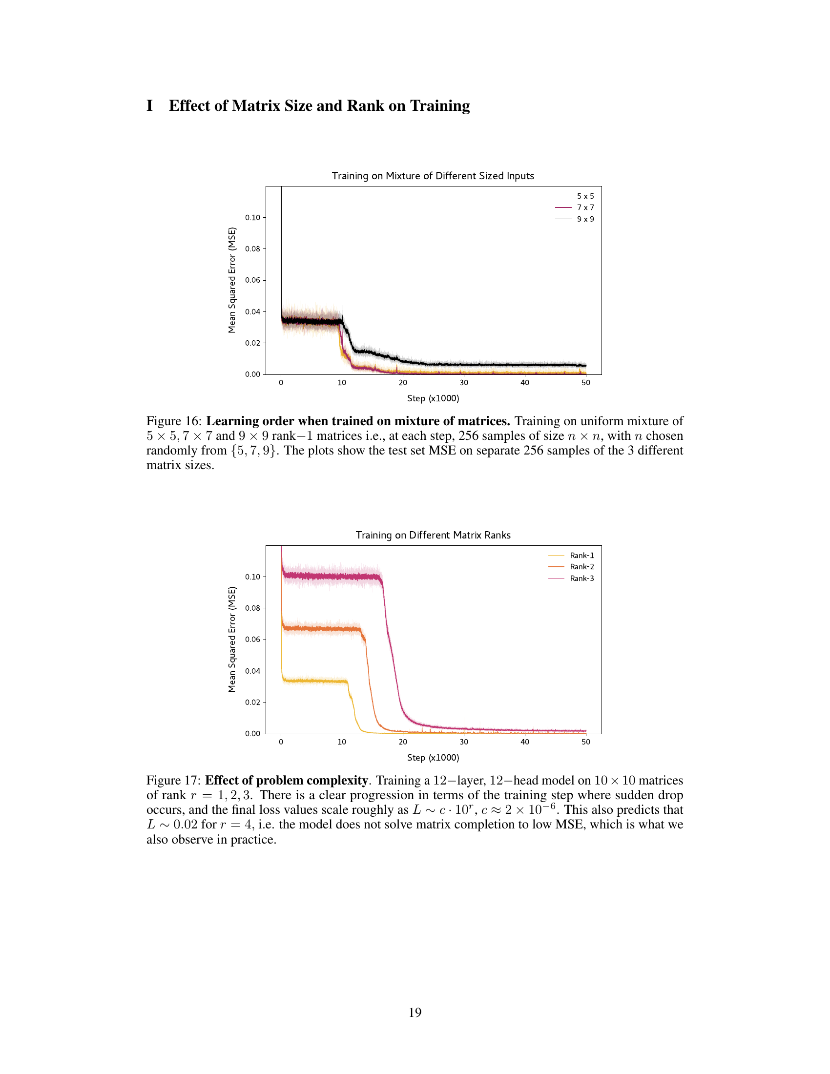
🔼 This figure shows the test set mean squared error (MSE) for matrix completion tasks with different input matrix sizes (5x5, 7x7, 9x9) over 50,000 training steps. The training data is a uniform mixture of these sizes. The plot demonstrates how the model’s performance on each size of matrix varies during training, indicating the learning order and generalization capabilities of the model.
read the caption
Figure 16: Learning order when trained on mixture of matrices. Training on uniform mixture of 5 × 5, 7 × 7 and 9 × 9 rank-1 matrices i.e., at each step, 256 samples of size n × n, with n chosen randomly from {5, 7, 9}. The plots show the test set MSE on separate 256 samples of the 3 different matrix sizes.

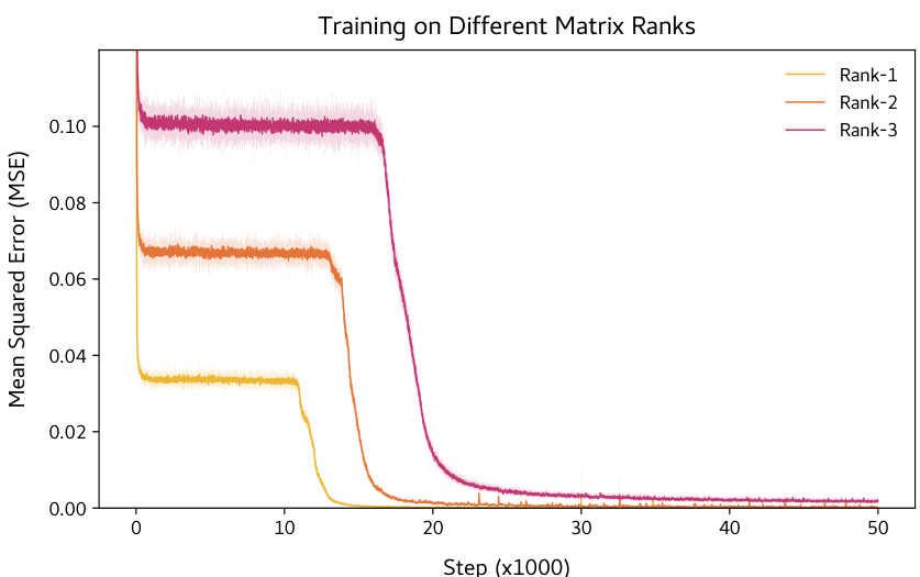
🔼 This figure shows the training loss dynamics of a BERT model trained on matrix completion. The loss initially plateaus for a significant number of training steps before suddenly dropping to near-optimal values. This abrupt drop illustrates the algorithmic transition described in the paper, where the model shifts from a copying strategy to an accurate matrix completion strategy.
read the caption
Figure 2: Sharp reduction in training loss.

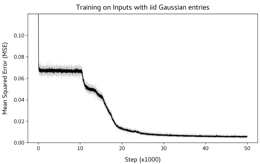
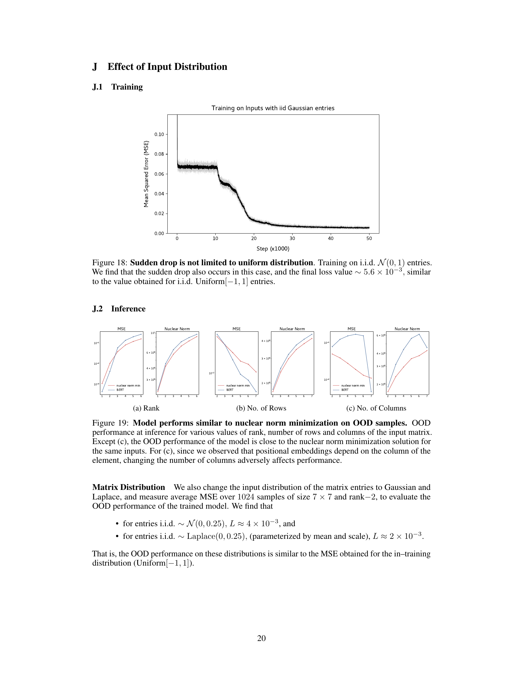
🔼 This figure shows the training loss curve for a BERT model trained on a matrix completion task where the input matrix entries are sampled from a Gaussian distribution with mean 0 and standard deviation 1. The key observation is that the sudden drop in training loss, a phenomenon observed in the paper with uniformly distributed inputs, also occurs in this setting. The final loss value is comparable to that achieved with uniformly distributed inputs, suggesting the robustness of the sudden drop phenomenon to the input data distribution.
read the caption
Figure 18: Sudden drop is not limited to uniform distribution. Training on i.i.d. N(0, 1) entries. We find that the sudden drop also occurs in this case, and the final loss value ~ 5.6 × 10⁻³, similar to the value obtained for i.i.d. Uniform[-1,1] entries.

🔼 This figure compares the performance of the BERT model and nuclear norm minimization on out-of-distribution (OOD) samples for matrix completion tasks. The plots show the mean squared error (MSE) and nuclear norm for varying ranks, number of rows, and number of columns in the input matrices. The results indicate that the BERT model’s performance closely matches that of nuclear norm minimization for most scenarios, with the exception of varying the number of columns. This exception highlights the impact of positional embeddings learned by the BERT model, demonstrating that its matrix completion approach isn’t a simple application of nuclear norm minimization.
read the caption
Figure 19: Model performs similar to nuclear norm minimization on OOD samples. OOD performance at inference for various values of rank, number of rows and columns of the input matrix. Except (c), the OOD performance of the model is close to the nuclear norm minimization solution for the same inputs. For (c), since we observed that positional embeddings depend on the column of the element, changing the number of columns adversely affects performance.

🔼 The figure shows the training loss dynamics of a BERT model trained on the matrix completion task. The loss starts high and remains relatively flat for a significant number of training steps (plateau phase). Then, there is a sharp and sudden drop in the loss to near optimal values (algorithmic shift). This sudden drop in loss is a key observation of the paper, and a focus of the interpretability analysis.
read the caption
Figure 2: Sharp reduction in training loss.

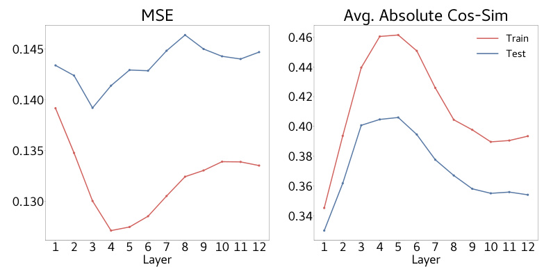
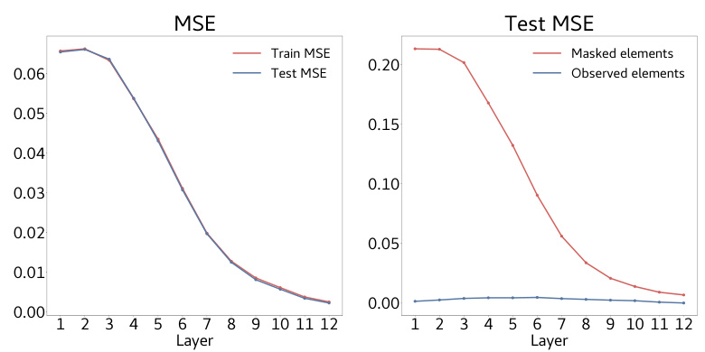
🔼 This figure shows the results of probing experiments to investigate how well the model’s hidden states encode information about the input matrix. Linear probes were used to predict the row of each element in the input matrix, with missing entries replaced by 0. The Mean Squared Error (MSE) and average absolute cosine similarity between the probe predictions and the actual values are plotted for each layer of the model. Layers 3 and 4 show significantly lower MSE and higher cosine similarity, indicating that these layers are particularly effective in encoding information about the masked input matrix.
read the caption
Figure 6: Hidden states encode input information. We probe for the row of each element in the masked matrix input, replacing missing entries by 0. We find that layers 3 and 4 have a much lower MSE and a much larger cosine similarity compared to other layers in the model. Hence, these layers somehow ‘store information’ about the masked input matrix.

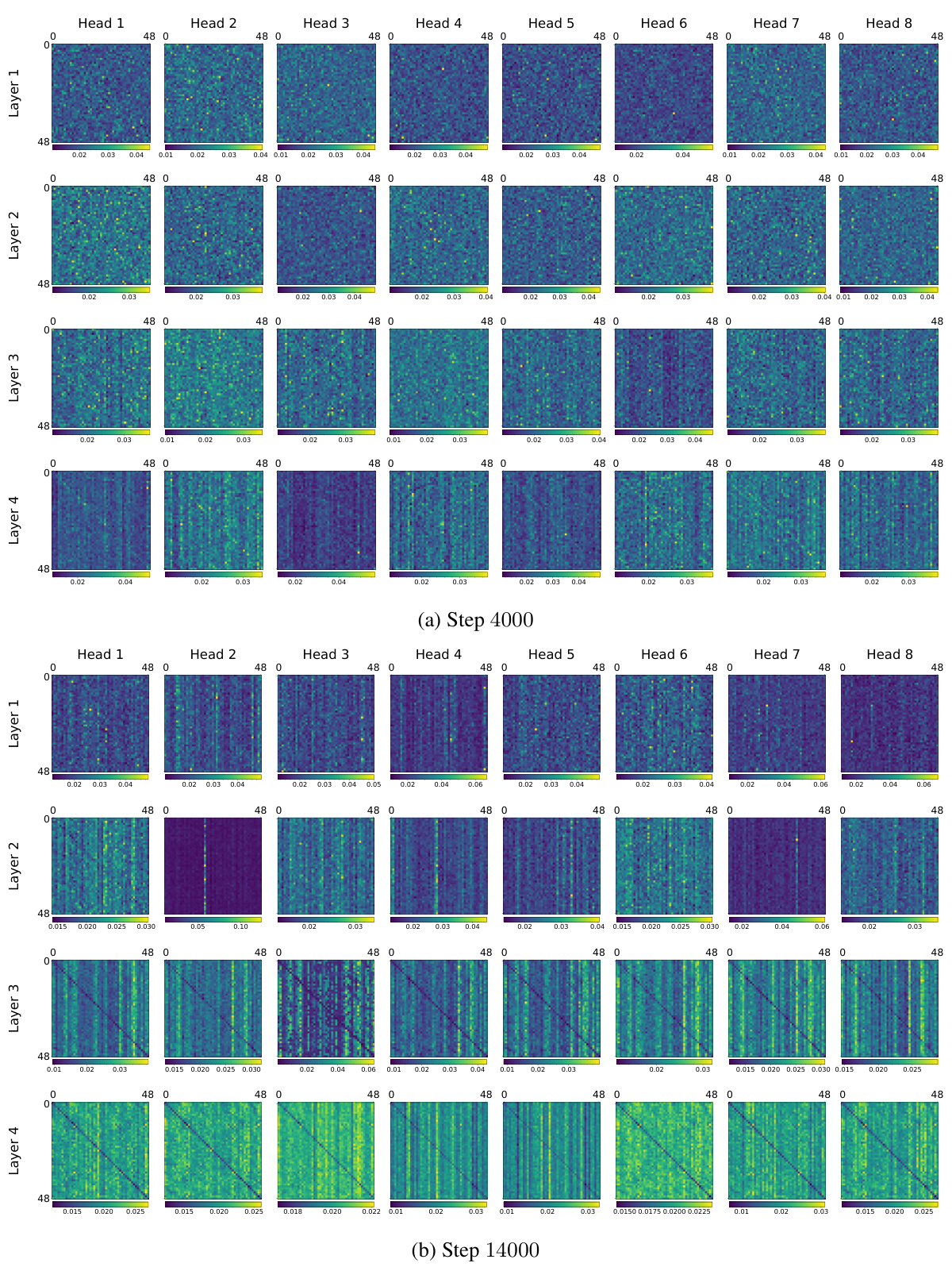
🔼 This figure visualizes the attention head weights at different training steps (4000, 14000, 16000, and 20000). Each subplot represents an attention head within a specific layer of the BERT model. The color intensity represents the attention weight, with brighter colors indicating stronger attention. The figure shows how attention patterns evolve as training progresses. It illustrates the change from non-interpretable patterns in early stages (pre-algorithmic shift) to clearly interpretable patterns (post-algorithmic shift) which show that the model is focusing on different parts of the input matrix, reflecting its progress in solving the matrix completion task.
read the caption
Figure 22: Attention heads across various training steps.

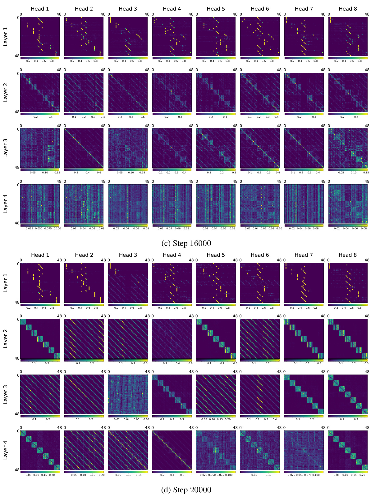
🔼 This figure shows the attention head weights across different layers of the BERT model at various training steps (4000, 14000, 16000, and 20000). Each layer is displayed as a matrix of attention weights for the eight attention heads. The change in the attention patterns across layers and different heads highlight the model’s transition from the copying phase to the computation phase in matrix completion. The change reflects how the model learns to focus on relevant parts of the input matrix during matrix completion.
read the caption
Figure 22: Attention heads across various training steps.

🔼 This figure shows the attention head weights across different layers of the model at various training steps. It visually represents how the attention mechanisms change over time, transitioning from seemingly random patterns early in training to more structured patterns later, which are relevant to the task of matrix completion. The changes in attention patterns correlate with the sudden drop in loss observed in the training curve, illustrating the model’s shift from simply copying input values to actively computing the missing elements.
read the caption
Figure 22: Attention heads across various training steps.

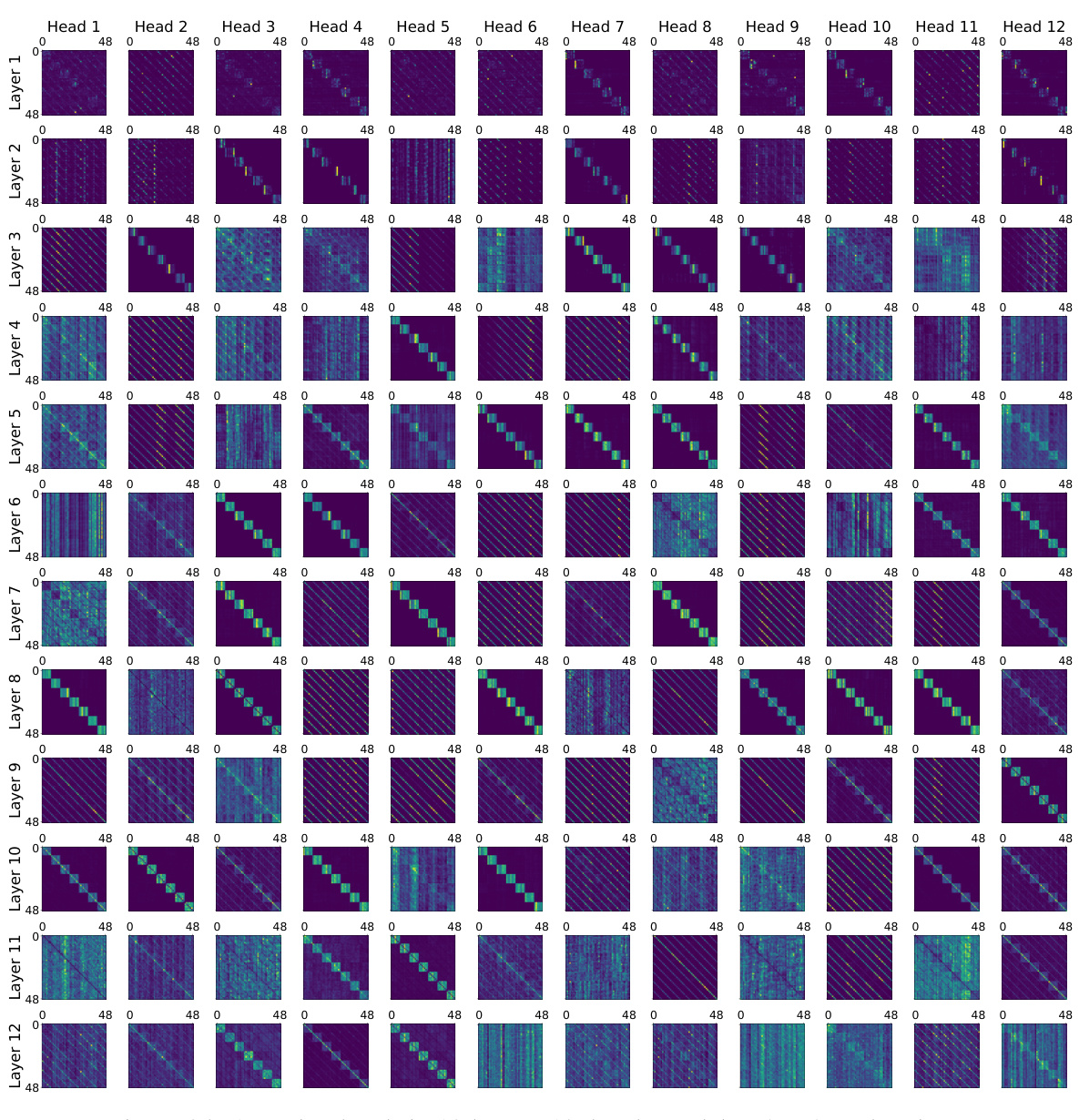
🔼 This figure visualizes the attention head weights across different layers of the BERT model at various training steps (4000, 14000, 16000, 20000). Each subfigure represents a specific training step and shows the attention weight matrices for all eight attention heads within each of the four layers of the BERT model. The color intensity represents the magnitude of attention weights, allowing for the visualization of how the attention patterns evolve during training. This evolution illustrates the shift in the model’s behavior from a copying phase to a completion phase, which is discussed in the paper.
read the caption
Figure 22: Attention heads across various training steps.

🔼 This figure visualizes the attention heads across different layers of the BERT model at various training steps (4000, 14000, 16000, 20000). Each sub-figure shows the attention weights for all heads within a specific layer. The color intensity represents the attention weight, with darker colors indicating stronger attention. The figure aims to demonstrate how the attention patterns evolve during training, transitioning from seemingly random patterns in the early stages to more structured patterns focused on relevant input tokens as the model learns to accurately complete the missing entries in the matrix completion task.
read the caption
Figure 22: Attention heads across various training steps.

🔼 This figure visualizes the attention head matrices at different stages of the model’s training. It shows how the attention patterns evolve from a largely unstructured state early in training (Step 4000) to more structured and interpretable patterns later in training (Steps 14000, 16000, and 20000). The changes in attention patterns are directly related to the model’s algorithmic transition from simply copying the input to accurately predicting the missing values, as described in the paper.
read the caption
Figure 22: Attention heads across various training steps.

TL;DR#

Key Takeaways#

Why does it matter?#

Visual Insights#

In-depth insights#

Abrupt Learning#

BERT Matrix#

Algorithmic Shift#

Model Dynamics#

Future Work#

More visual insights#

Full paper#