TL;DR#
Many AI applications rely on ranking problems, and the Average Top-k (ATk) loss is often used to address imbalanced datasets. However, ATk requires computationally expensive sorting algorithms. This paper tackles the inefficiency by introducing STk, a novel, fully differentiable module that addresses Top-k problems directly and efficiently within a unified computational graph. STk avoids sorting, significantly improving speed.
The proposed STk loss, which incorporates STk, outperforms ATk loss on multiple benchmarks, exhibiting superior average performance and lower standard deviation. This improvement extends to real-world scenarios, as demonstrated by surpassing state-of-the-art results on CIFAR-100-LT and Places-LT leaderboards. The authors also explore applications for STk in different learning tasks and demonstrate its scalability and efficiency.
Key Takeaways#
Why does it matter?#
This paper is important because it introduces STk, a novel and efficient module that significantly speeds up the computation of Top-k problems in deep learning, a common yet computationally expensive task. This has major implications for various applications, such as imbalanced classification and long-tailed learning, where it leads to improved accuracy and efficiency. Furthermore, the fully differentiable nature of STk enables its seamless integration into existing neural networks, paving the way for wider adoption and further research on Top-k optimization.
Visual Insights#
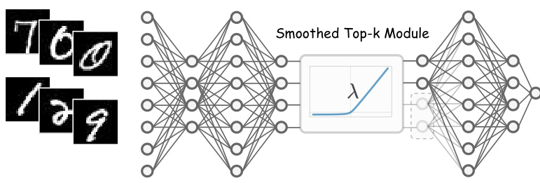
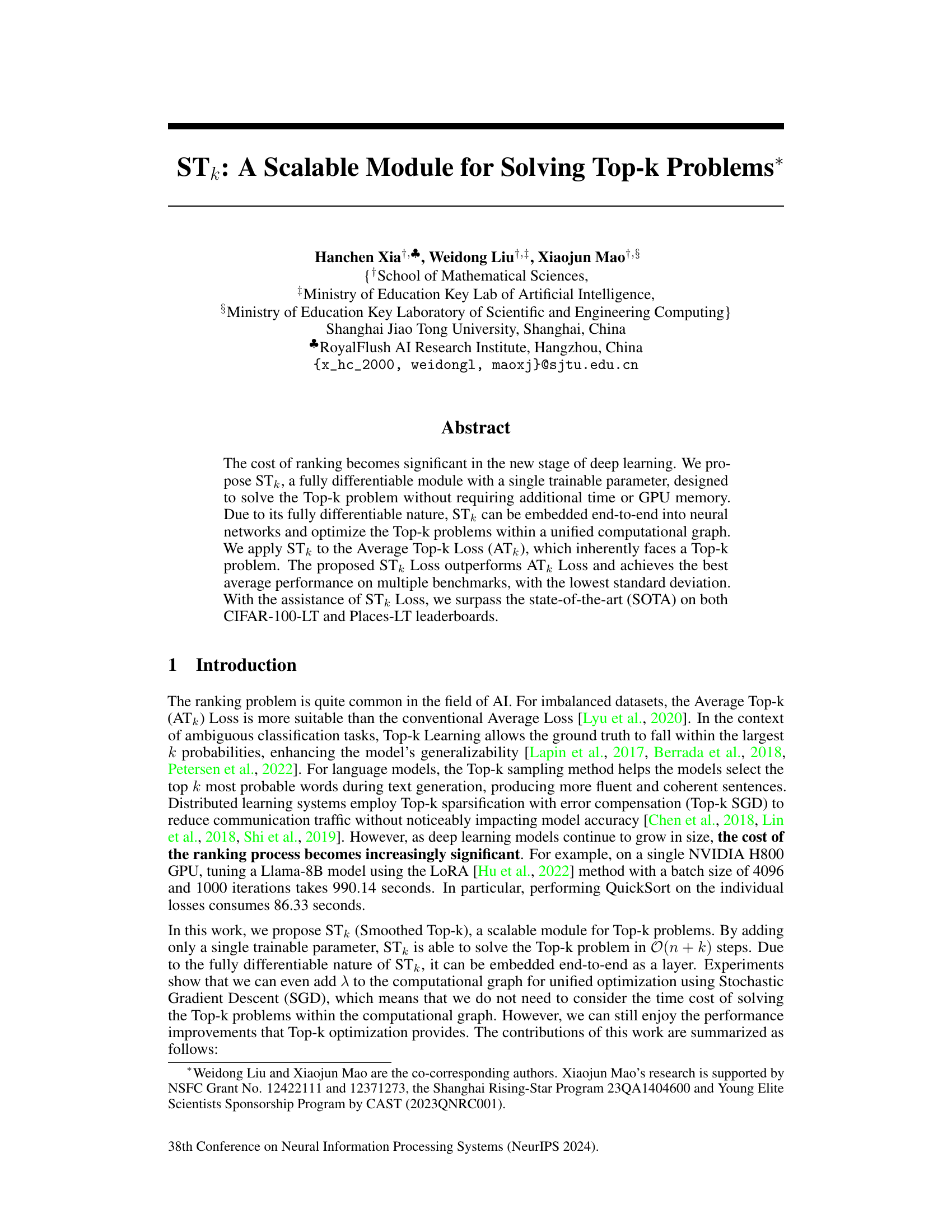
🔼 This figure illustrates the architecture of the Smoothed Top-k (STk) module. The STk module is designed to be inserted into any layer of a neural network to efficiently solve the Top-k problem. The module utilizes a single trainable parameter, λ (lambda), which dynamically approximates the k-th largest element within a set of elements. This approximation allows for the selection of the top-k elements without requiring computationally expensive sorting algorithms, making the process differentiable and efficient within the neural network’s computational graph. The diagram shows the STk module integrated between two fully-connected layers, highlighting its seamless integration into existing network structures. The graph to the right of the module illustrates the smoothed approximation function used.
read the caption
Figure 1: STk Architecture. For any layer of neurons in a neural network, to solve the Top-k problem for its weights, insert an STk Module. The trainable parameter λ will gradually approximate the k-th largest element during the optimization process. And this λ can be used to filter neurons.
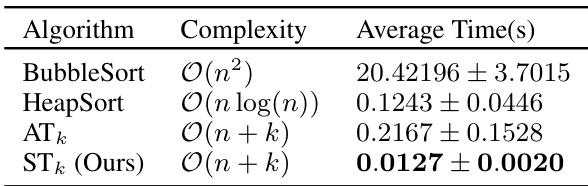
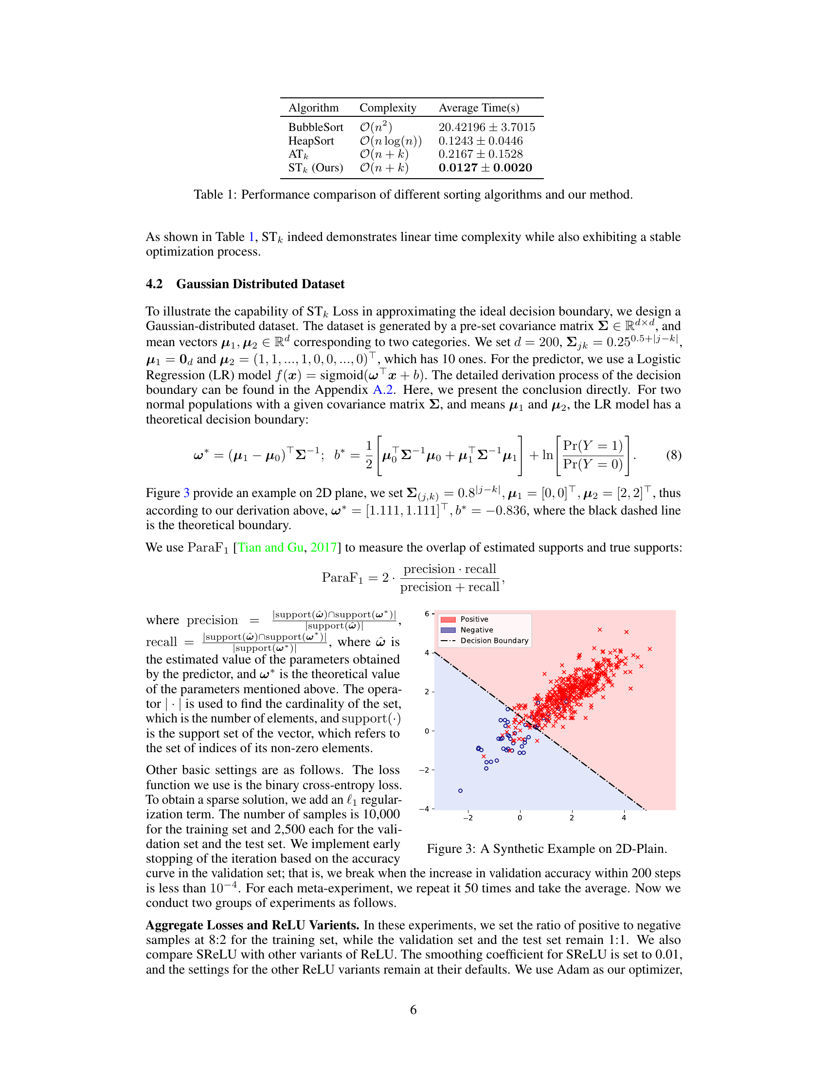
🔼 This table compares the average time taken by different sorting algorithms (BubbleSort, HeapSort, ATk) and the proposed STk method to solve the Top-k problem. The time is measured in seconds and represents the average of 50 experiments. The results demonstrate that STk achieves linear time complexity while maintaining stability, significantly outperforming other methods.
read the caption
Table 1: Performance comparison of different sorting algorithms and our method.
In-depth insights#
Smoothed Top-k#
The concept of “Smoothed Top-k” suggests a method for efficiently and differentiably solving top-k problems within neural networks. Traditional top-k operations often involve sorting, a non-differentiable process that hinders end-to-end training. The “smoothing” aspect likely involves approximating the non-differentiable parts of the top-k selection process using a smooth, differentiable function. This allows the algorithm to be seamlessly integrated into the backpropagation process, enabling gradient-based optimization. A key advantage is the potential for significant speed improvements over traditional methods, as sorting algorithms generally have a higher time complexity than the proposed smoothed approach. The single trainable parameter further suggests an efficient and easily implemented method. The effectiveness of the method likely relies heavily on the choice of smoothing function and its ability to accurately approximate the top-k selection while maintaining differentiability. The tradeoff between accuracy and computational efficiency is a crucial aspect of this technique; a good smoothing function should balance both. Overall, “Smoothed Top-k” aims to address a critical limitation in deep learning, improving the efficiency and practicality of handling top-k problems in various applications.
ATk Loss#
The Average Top-k (ATk) loss function is designed to address the limitations of traditional average loss, particularly in scenarios with imbalanced datasets or ambiguous classifications. Unlike average loss, which can be heavily skewed by a few large losses, ATk focuses on the k largest losses, providing a more robust measure of model performance. This robustness makes ATk particularly useful in the context of long-tailed learning, where data scarcity in certain classes can disproportionately inflate the average loss. By focusing on the most significant losses, ATk prevents these tail classes from dominating the overall loss calculation, allowing for improved model generalizability. The parameter ‘k’ in ATk is a hyperparameter that needs to be carefully tuned based on the specific dataset and task. A larger k may capture more of the data distribution, but it could also result in less sensitivity to outlier errors. A fully differentiable implementation of ATk, however, requires computationally expensive sorting algorithms, making it less scalable for large datasets. This is where the proposed STk Loss addresses the shortcomings. The paper’s key contribution appears to be a differentiable and computationally efficient approximation of ATk, improving scalability and performance in the context of neural network training.
STk Loss#
The proposed STk Loss is a novel approach to address the limitations of existing top-k loss functions, particularly the Average Top-k (ATk) Loss. STk Loss leverages a smoothed Top-k module (STk), which efficiently approximates the k-th largest element without the computational overhead of sorting algorithms. This efficiency is crucial for large-scale deep learning applications, and unlike ATk loss, it does not require extra computation time or GPU memory. The fully differentiable nature of STk allows for end-to-end optimization within neural networks, simplifying the training process. Experimental results across various benchmarks demonstrate that STk Loss consistently outperforms ATk Loss and achieves state-of-the-art performance on long-tailed image classification datasets. The key innovation lies in the smooth approximation of the ReLU function, which resolves the non-differentiability issues inherent in previous Top-k optimization approaches. The superior performance and computational efficiency of STk Loss strongly suggest its potential as a valuable tool in various machine learning tasks.
Imbalanced Datasets#
Imbalanced datasets, where one class significantly outnumbers others, pose a substantial challenge in machine learning. Standard classification algorithms often perform poorly on the minority class, leading to inaccurate and misleading models. Addressing this necessitates techniques beyond simple class weighting. Resampling strategies, such as oversampling the minority class or undersampling the majority, can help balance the dataset, but these methods can introduce bias or lose valuable data. Cost-sensitive learning assigns different misclassification costs to different classes, penalizing errors on the minority class more heavily. Ensemble methods, like bagging or boosting, combined with techniques focused on imbalanced data, provide enhanced robustness. Advanced techniques such as anomaly detection can effectively identify the minority class, especially if it’s considered an outlier. Choosing appropriate evaluation metrics, beyond simple accuracy (e.g., precision, recall, F1-score, AUC), is crucial for a fair assessment of model performance on imbalanced data. Successfully handling imbalanced datasets often involves a combination of these methods tailored to the specific characteristics of the problem and dataset.
Future Work#
The ‘Future Work’ section of this research paper could explore several promising directions. Extending STk to handle more complex Top-k problems beyond simple ranking tasks is crucial. This might involve adapting STk for scenarios with weighted elements, dynamically changing k values, or more intricate ranking criteria. Investigating the theoretical properties of STk more deeply, such as its convergence rate under different optimization algorithms and its robustness to noise, would provide a solid foundation for broader applications. A critical area for future work is a comprehensive empirical evaluation across a wider range of datasets and tasks. This includes exploring diverse application domains such as natural language processing, time series analysis, and recommender systems. Furthermore, exploring the integration of STk with other techniques for addressing long-tailed distributions or imbalanced data is important. Finally, the potential benefits of exploring different smoothing functions beyond SReLU and a detailed comparison of their performance and convergence characteristics deserve attention. These future research directions would strengthen the paper’s contribution and broaden the applicability of the proposed STk module.
More visual insights#
More on figures
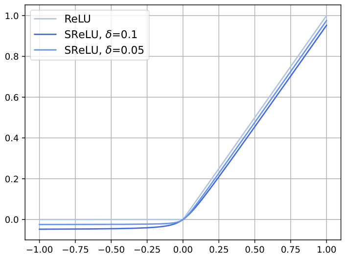
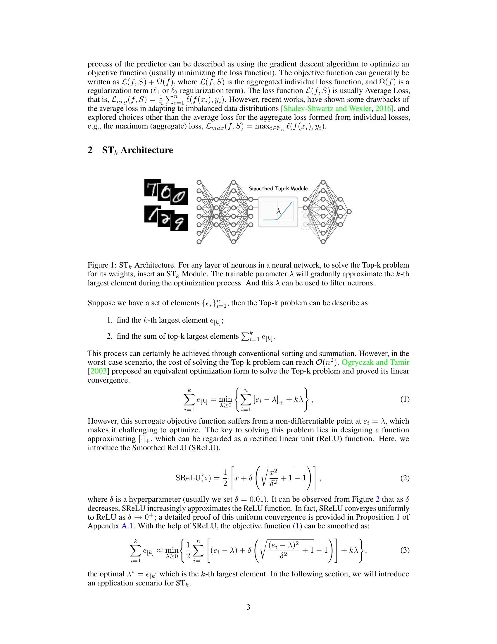
🔼 This figure compares the ReLU (Rectified Linear Unit) activation function with the smoothed ReLU (SReLU) function for different smoothing coefficients (δ). The SReLU function is a smooth approximation of the ReLU function, which is non-differentiable at x = 0. As the smoothing coefficient (δ) decreases, the SReLU function increasingly approximates the ReLU function, demonstrating its uniform convergence to ReLU as δ approaches 0. This is important because the SReLU function’s differentiability allows for easier optimization in neural networks.
read the caption
Figure 2: ReLU and SReLU with various smoothing coefficients δ.

🔼 This figure compares the ReLU (Rectified Linear Unit) activation function with the smoothed ReLU (SReLU) activation function. The SReLU function is a smoothed approximation of the ReLU function, designed to be differentiable everywhere. The figure shows how the SReLU function approaches the ReLU function as the smoothing coefficient (δ) decreases. This is important because the SReLU function is used within the STk module described in the paper to make the Top-k operation fully differentiable.
read the caption
Figure 2: ReLU and SReLU with various smoothing coefficients δ.
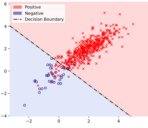
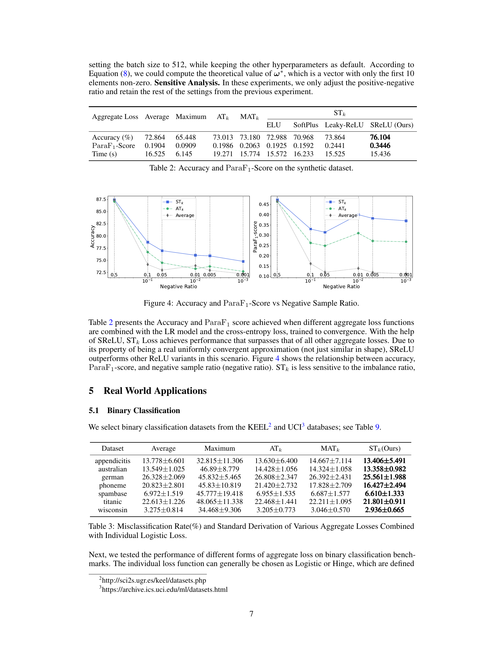
🔼 This figure shows a synthetic example on a 2D plane to illustrate the capability of the STk loss in approximating the ideal decision boundary. It displays a scatter plot of data points belonging to two categories (positive and negative), colored red and blue respectively. A decision boundary line separates the two categories, visually demonstrating how well a model trained with STk loss approximates this theoretical boundary.
read the caption
Figure 3: A Synthetic Example on 2D-Plain.
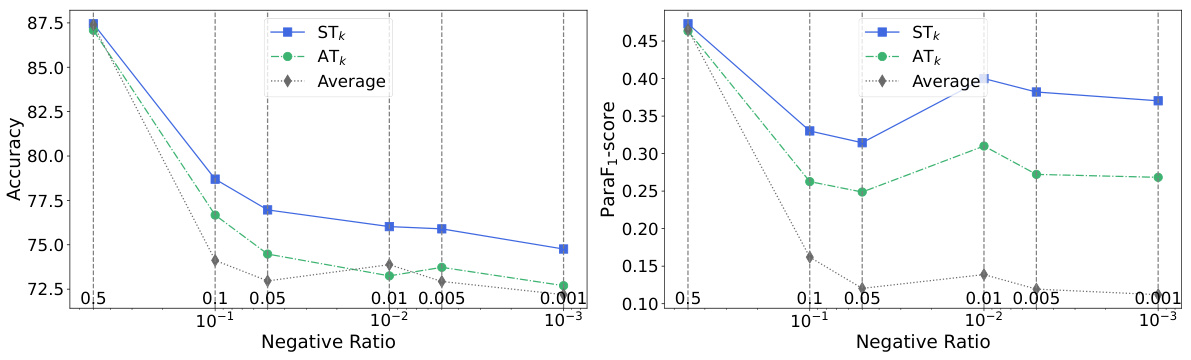
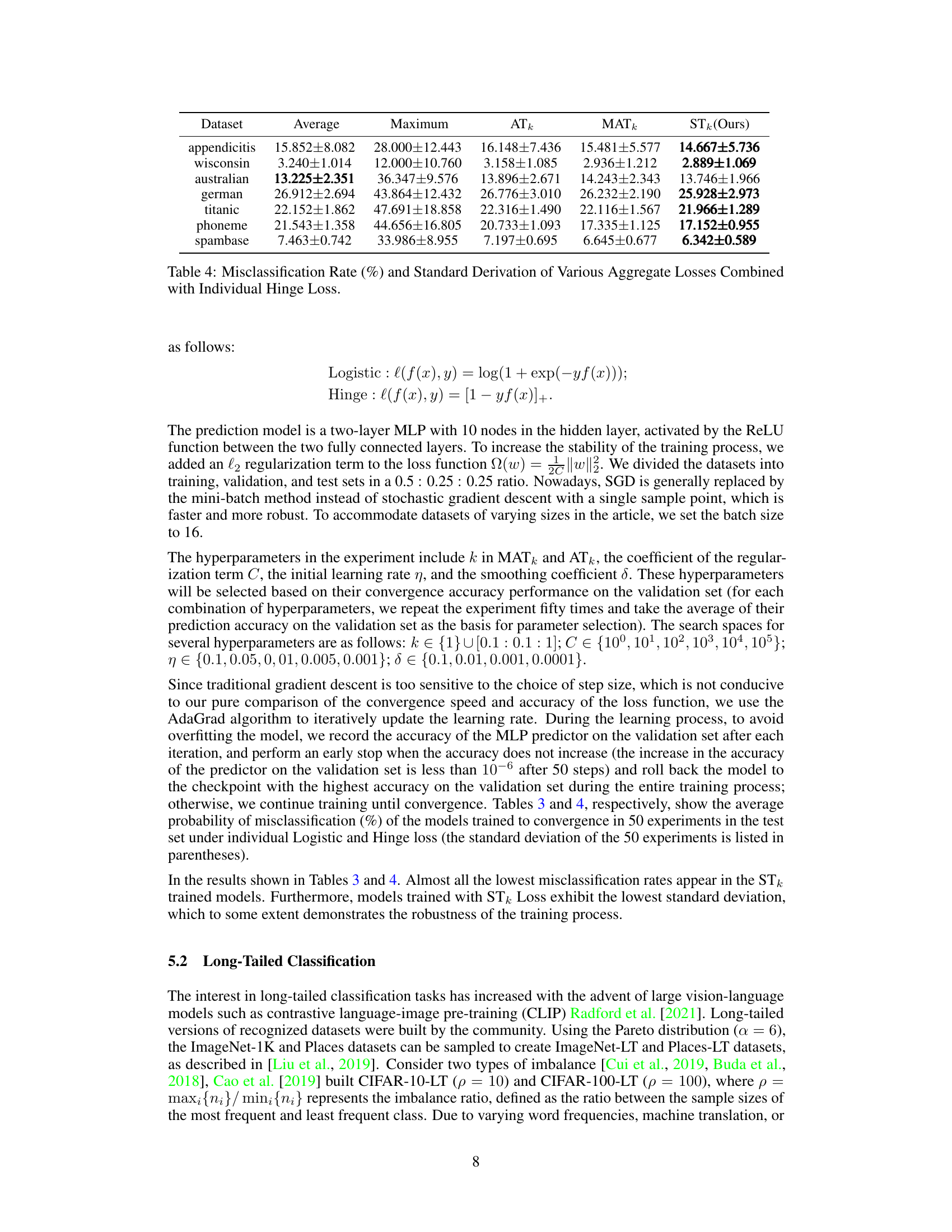
🔼 This figure shows the performance of different aggregate loss functions (STk, ATk, Average) under varying negative sample ratios. The x-axis represents the negative sample ratio, while the y-axis shows both the accuracy and ParaF1-score. It demonstrates how the performance of each method changes as the class imbalance increases. STk consistently outperforms ATk and Average across all negative ratios, showing its robustness to class imbalance.
read the caption
Figure 4: Accuracy and ParaF1-Score vs Negative Sample Ratio.
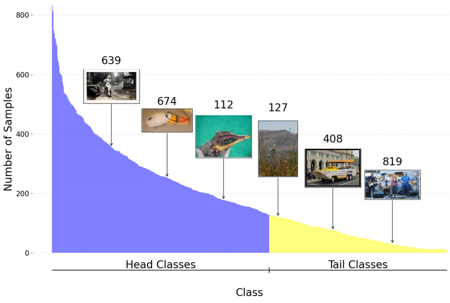
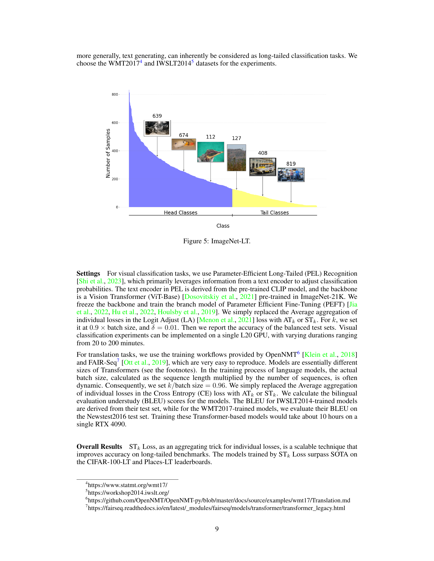
🔼 This figure shows the class distribution in the ImageNet-LT dataset. The x-axis represents the classes, and the y-axis represents the number of samples per class. The dataset is highly imbalanced; a few classes (head classes) have many samples while most classes (tail classes) have very few samples. Representative images are shown for some of the head and tail classes, illustrating the variety of images found within each class.
read the caption
Figure 5: ImageNet-LT.
More on tables
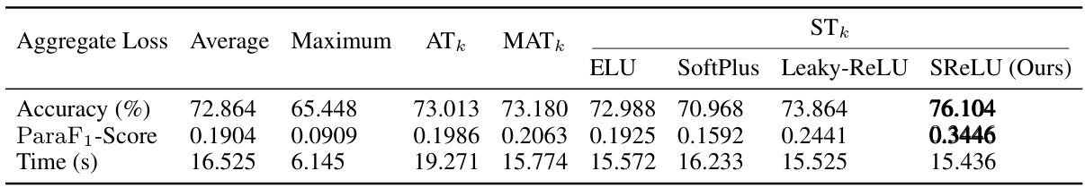
🔼 This table presents the accuracy and ParaF1 score achieved when different aggregate loss functions are combined with the LR model and the cross-entropy loss, trained to convergence. It shows the results for Average, Maximum, ATk, MATk losses, and for the proposed STk loss with different ReLU variants (ELU, SoftPlus, Leaky-ReLU, and SReLU). The table also shows the computation time taken by each method.
read the caption
Table 2: Accuracy and ParaF1-Score on the synthetic dataset.
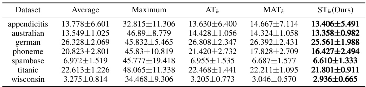
🔼 This table presents the results of a binary classification experiment comparing different aggregate loss functions combined with individual logistic loss. The misclassification rate and its standard deviation are reported for various datasets using Average, Maximum, ATk, MATk and the proposed STk loss functions. The results illustrate the performance improvement achieved by using STk Loss, especially in terms of reducing the standard deviation of the error rate.
read the caption
Table 3: Misclassification Rate(%) and Standard Derivation of Various Aggregate Losses Combined with Individual Logistic Loss.
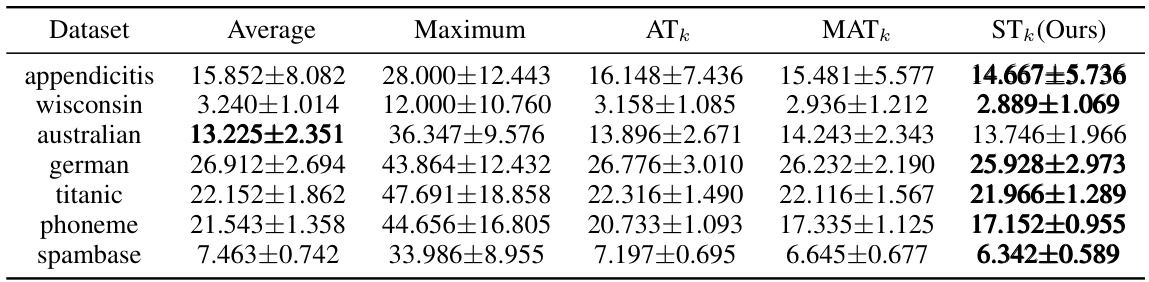
🔼 This table presents the results of experiments comparing different aggregate loss functions (Average, Maximum, ATk, MATk, and STk) combined with the individual Hinge loss for binary classification tasks. The misclassification rate and standard deviation are shown for several datasets (appendicitis, wisconsin, australian, german, titanic, phoneme, spambase). The STk method consistently shows either the lowest or a near-lowest misclassification rate and often demonstrates the lowest standard deviation, indicating improved stability and robustness.
read the caption
Table 4: Misclassification Rate (%) and Standard Derivation of Various Aggregate Losses Combined with Individual Hinge Loss.
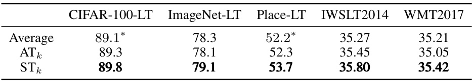
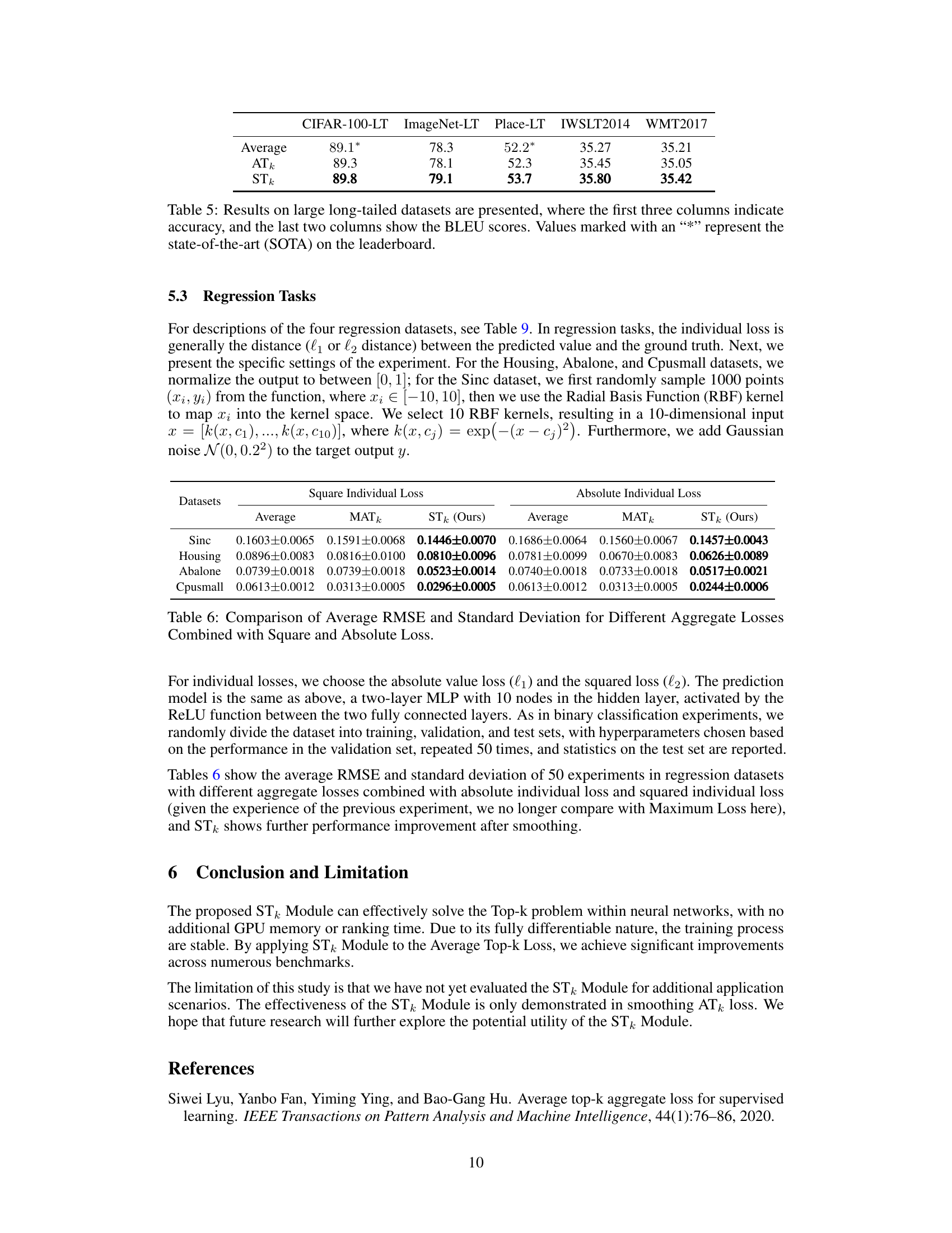
🔼 This table presents the results of the proposed STk method on several large, long-tailed datasets. The first three columns show the accuracy achieved on CIFAR-100-LT, ImageNet-LT, and Places-LT, respectively. The last two columns display the BLEU scores obtained for machine translation tasks on IWSLT2014 and WMT2017 datasets. The results demonstrate that the STk method surpasses the state-of-the-art (indicated by ‘*’) on several benchmarks.
read the caption
Table 5: Results on large long-tailed datasets are presented, where the first three columns indicate accuracy, and the last two columns show the BLEU scores. Values marked with an '*' represent the state-of-the-art (SOTA) on the leaderboard.

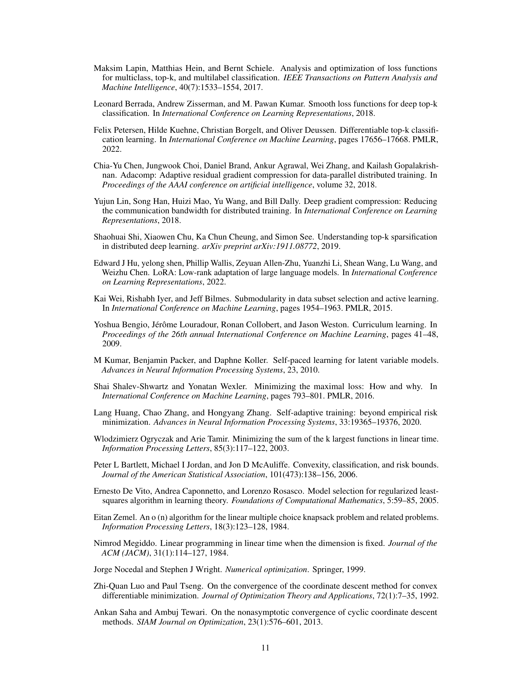
🔼 This table presents a comparison of the root mean squared error (RMSE) and standard deviation for different aggregate loss functions (Average, MATk, and STk) combined with both square and absolute individual losses. The results are shown for four different regression datasets (Sinc, Housing, Abalone, and Cpusmall). It demonstrates the performance of the proposed STk loss compared to other aggregation methods.
read the caption
Table 6: Comparison of Average RMSE and Standard Deviation for Different Aggregate Losses Combined with Square and Absolute Loss.
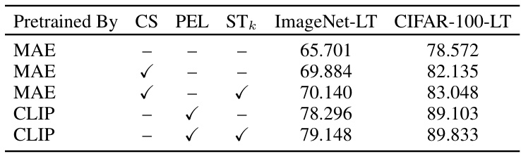
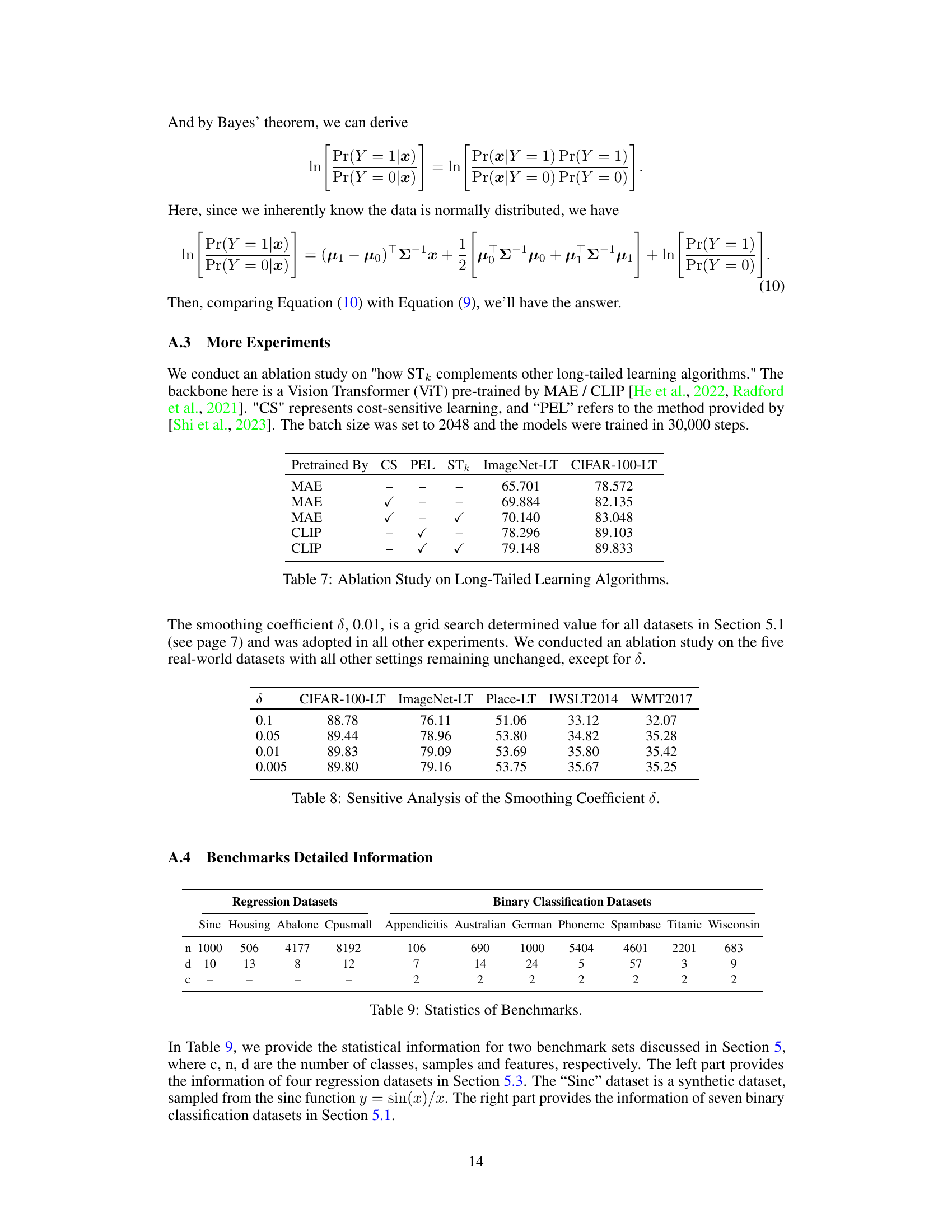
🔼 This table presents the results of an ablation study on long-tailed learning algorithms. It shows the performance (accuracy on ImageNet-LT and CIFAR-100-LT datasets) achieved by using different combinations of techniques: MAE or CLIP pre-training, cost-sensitive learning (CS), Parameter-Efficient Long-Tailed (PEL) Recognition, and the proposed Smoothed Top-k (STk) module. The table helps to understand the individual and combined contributions of these methods to improving the performance on long-tailed image classification tasks.
read the caption
Table 7: Ablation Study on Long-Tailed Learning Algorithms.

🔼 This table presents the results of an ablation study on the smoothing coefficient (δ) used in the STk loss function. It shows how the performance metrics (accuracy for image classification datasets and BLEU score for translation datasets) vary across different values of δ on five real-world datasets: CIFAR-100-LT, ImageNet-LT, Place-LT, IWSLT2014, and WMT2017. The purpose is to demonstrate the sensitivity of the model’s performance to this hyperparameter and identify an optimal or near-optimal value of δ. The results help to demonstrate the robustness of STk loss to small variations in the choice of δ.
read the caption
Table 8: Sensitive Analysis of the Smoothing Coefficient δ.
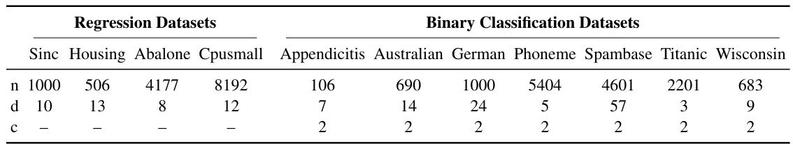
🔼 This table provides a detailed statistical overview of the datasets used in the paper’s experiments. It includes the number of samples (n), features (d), and classes (c) for both regression and binary classification datasets. The regression datasets are Sinc, Housing, Abalone, and Cpusmall, while the binary classification datasets are Appendicitis, Australian, German, Phoneme, Spambase, Titanic, and Wisconsin.
read the caption
Table 9: Statistics of Benchmarks.
Full paper#