TL;DR#
Modeling marked point processes typically relies on computationally expensive thinning algorithms. This poses challenges for real-time applications and long-horizon predictions. Existing neural-based models often depend on such computationally intensive methods, resulting in performance bottlenecks.
The proposed Decomposable Transformer Point Process (DTPP) model avoids this issue by employing an intensity-free approach. DTPP decomposes the problem, using a mixture of log-normals to model inter-event times and a Transformer-based architecture to model marks. This strategy greatly enhances computational efficiency. Empirical evaluations on real-world datasets demonstrate DTPP’s superior performance, achieving state-of-the-art results on next-event prediction and the more challenging long-horizon prediction tasks with a fraction of the inference time required by existing methods.
Key Takeaways#
Why does it matter?#
This paper is crucial for researchers working with temporal point processes. It offers a computationally efficient alternative to traditional methods, significantly improving inference speed. This opens avenues for real-world applications previously hindered by computational constraints, and introduces a novel, intensity-free modeling approach.
Visual Insights#
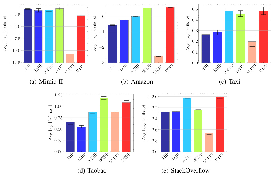
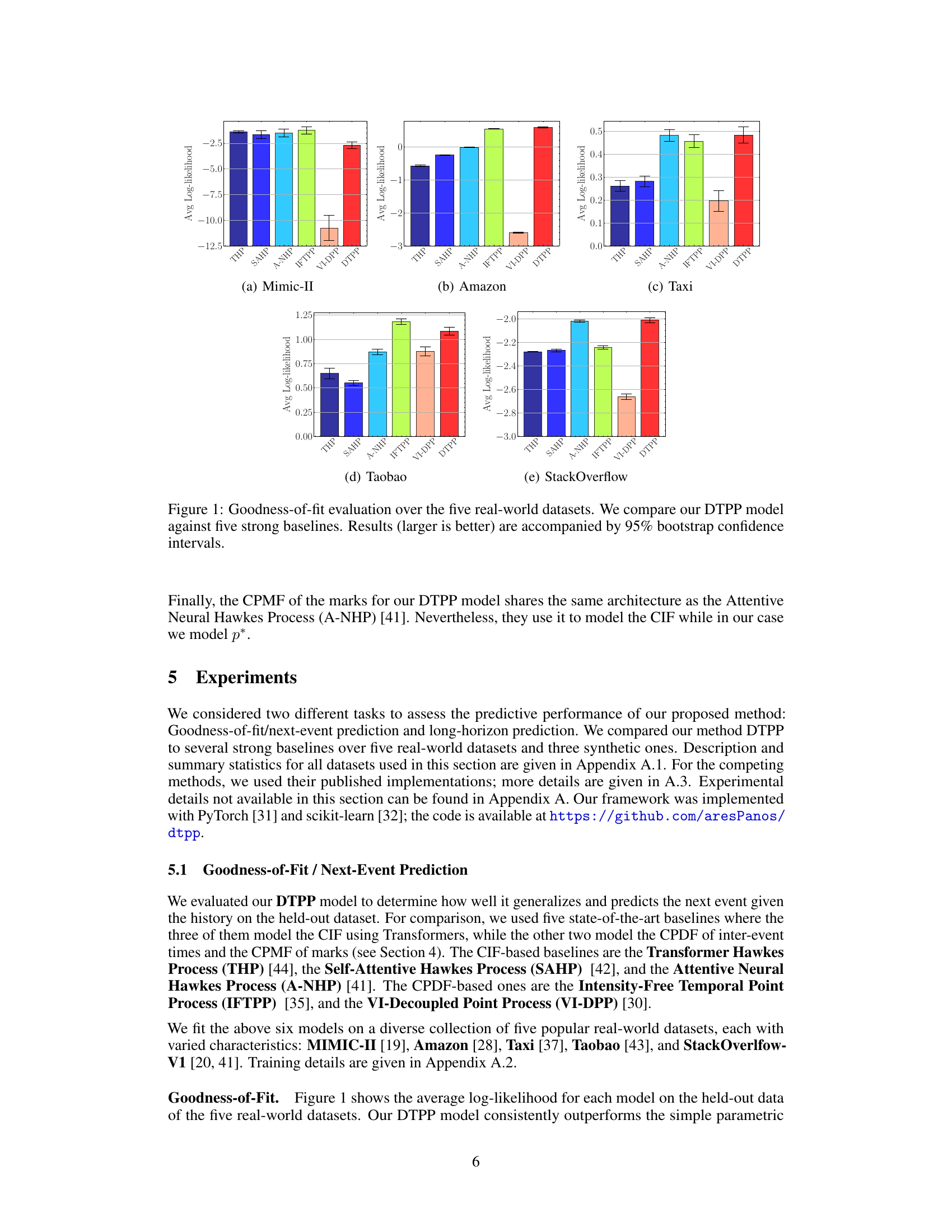
🔼 The figure compares the goodness-of-fit performance of the proposed Decomposable Transformer Point Process (DTPP) model against five other state-of-the-art models on five real-world datasets. The goodness-of-fit is measured using average log-likelihood. The results show that DTPP outperforms the baselines across most datasets, indicating its superior ability to model the data.
read the caption
Figure 1: Goodness-of-fit evaluation over the five real-world datasets. We compare our DTPP model against five strong baselines. Results (larger is better) are accompanied by 95% bootstrap confidence intervals.

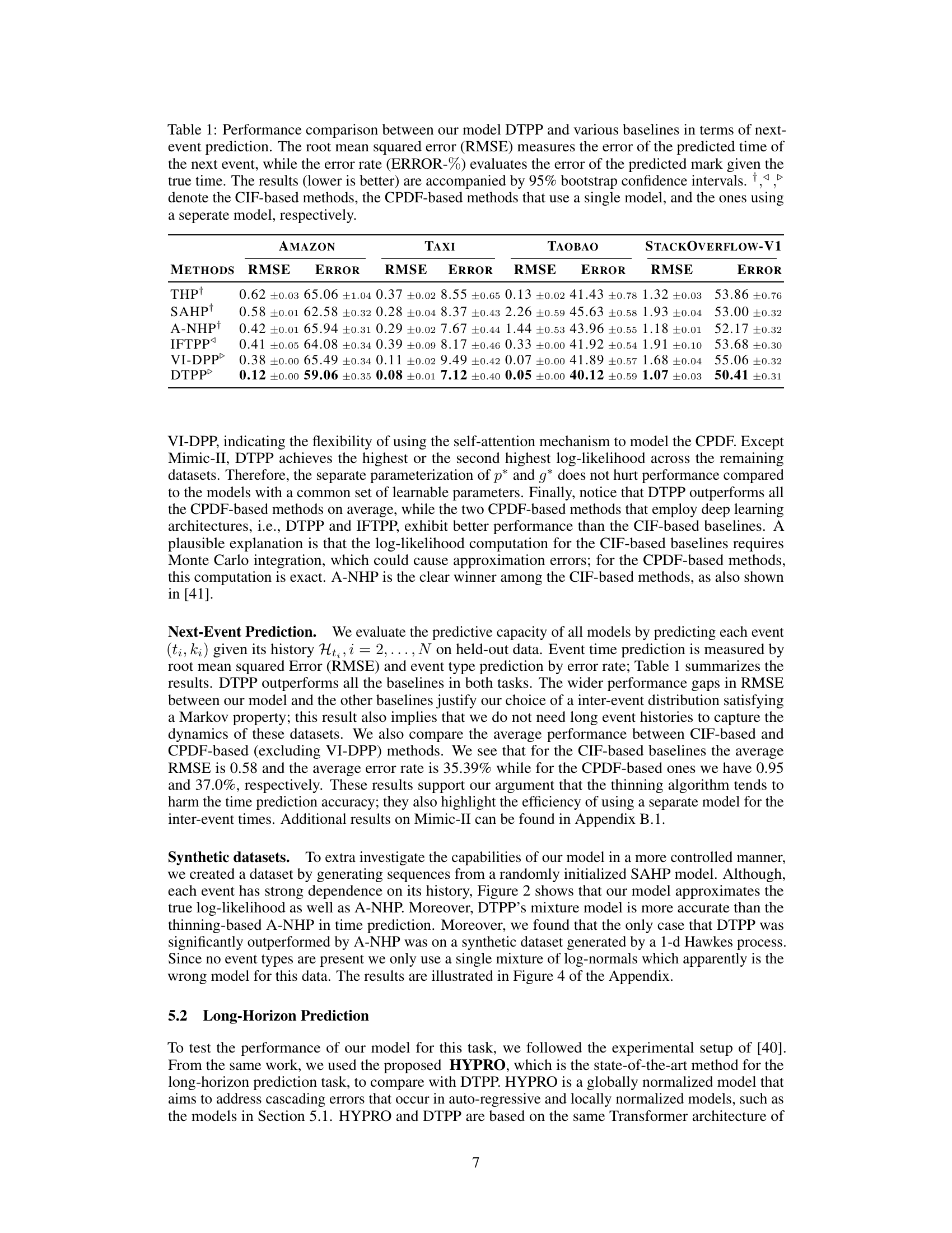
🔼 This table compares the performance of the proposed Decomposable Transformer Point Process (DTPP) model against other state-of-the-art models for next-event prediction. The evaluation metrics are Root Mean Squared Error (RMSE) for time prediction and Error Rate for mark prediction. Lower values indicate better performance. The table also categorizes models based on their approach (CIF-based, single-model CPDF-based, separate-model CPDF-based).
read the caption
Table 1: Performance comparison between our model DTPP and various baselines in terms of next-event prediction. The root mean squared error (RMSE) measures the error of the predicted time of the next event, while the error rate (ERROR-%) evaluates the error of the predicted mark given the true time. The results (lower is better) are accompanied by 95% bootstrap confidence intervals. 1,4,▷ denote the CIF-based methods, the CPDF-based methods that use a single model, and the ones using a seperate model, respectively.
In-depth insights#
DTPP Framework#
The Decomposable Transformer Point Process (DTPP) framework offers a novel approach to modeling marked point processes by decoupling the modeling of event times and marks. This decomposition avoids the computationally expensive thinning algorithm, a common bottleneck in traditional intensity-based methods. DTPP leverages a mixture of log-normals to model the distribution of inter-event times, effectively capturing temporal dependencies with a Markov assumption. Simultaneously, it utilizes a Transformer architecture to model the conditional probability mass function of the marks, allowing for the incorporation of rich contextual information from the event history. This dual approach results in a computationally efficient model that achieves state-of-the-art performance in various prediction tasks, including next-event and long-horizon prediction. The framework’s modularity makes it highly adaptable, with the potential for further enhancements through alternative distributions and neural architectures. The intensity-free nature of DTPP is a key strength, allowing for more straightforward inference and improved predictive power. This framework offers a significant advance in the modeling of marked point processes, enabling more efficient and accurate modeling of complex real-world event data.
Intensity-Free Inference#
Intensity-free inference in point process modeling offers a compelling alternative to traditional thinning-based methods. Thinning is computationally expensive, especially for complex models and long sequences. Intensity-free approaches avoid this bottleneck by directly modeling the probability distributions of inter-event times and marks, thus enabling faster and more efficient inference. This is particularly valuable for real-time applications or scenarios with extensive data, where thinning becomes computationally prohibitive. However, intensity-free methods might require more sophisticated modeling of the conditional distributions, which could lead to increased model complexity and potential challenges in parameter estimation. The trade-off between computational efficiency and model complexity needs careful consideration when choosing between intensity-free and thinning-based approaches. The choice depends heavily on the specific application and data characteristics. Future research could explore hybrid methods combining the strengths of both techniques to balance accuracy and efficiency.
Long-Horizon Prediction#
Long-horizon prediction in temporal point processes presents a unique challenge: accurately forecasting sequences of events far into the future. Traditional methods often struggle due to compounding errors; an initial misprediction cascades, impacting subsequent forecasts. The paper investigates this challenge, contrasting methods that rely on computationally intensive thinning algorithms with those that don’t. The intensity-free approach, avoiding thinning, demonstrates significant advantages in computational efficiency and potentially improved accuracy. The key insight lies in decoupling the modeling of inter-event times (using a Markov property for computational tractability) and event marks (leveraging the power of transformer architectures). This decomposition allows for efficient, parallel inference which is crucial for long-horizon prediction. Experiments showcase the effectiveness of this approach against strong baselines, highlighting the limitations of thinning-based methods and confirming the suitability of the proposed method for long-range temporal forecasting. The study highlights the trade-offs between modeling complexity and computational cost, particularly relevant in scenarios requiring real-time predictions.
Model Limitations#
The model’s reliance on a Markov property for inter-event times, while computationally efficient, might oversimplify complex temporal dependencies. The log-normal mixture model, though flexible, may struggle to capture intricate distributions found in real-world data, potentially leading to inaccuracies in predictions, especially for long-horizon forecasting. The Transformer architecture used for modeling marks, while powerful, demands substantial training data. Limited data could hinder performance and lead to overfitting. Furthermore, the model’s efficiency depends heavily on parallel processing, which might not be accessible to all users. While the decomposition of the likelihood function avoids thinning algorithms, the separate parameterization of marks and times might miss interactions between the two which an intensity function-based approach could capture.
Future Extensions#
Future work could explore several promising directions. Improving the model’s efficiency for long-horizon prediction is crucial, potentially through more efficient attention mechanisms or alternative model architectures. Extending the model to handle more complex event types and mark distributions would increase its applicability. Incorporating external information such as user preferences or social network interactions could further enhance predictive accuracy. Furthermore, developing methods for uncertainty quantification and incorporating causal inference techniques would be valuable additions. Finally, exploring applications to other domains like healthcare or finance, where continuous-time event data are prevalent, presents exciting opportunities.
More visual insights#
More on figures
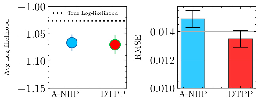
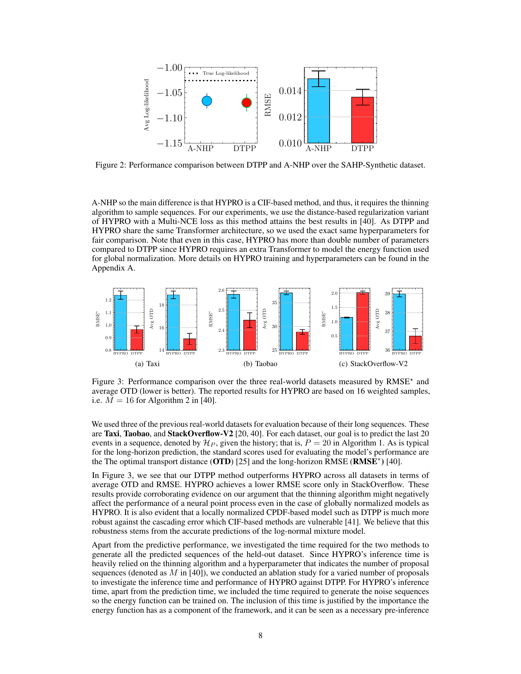
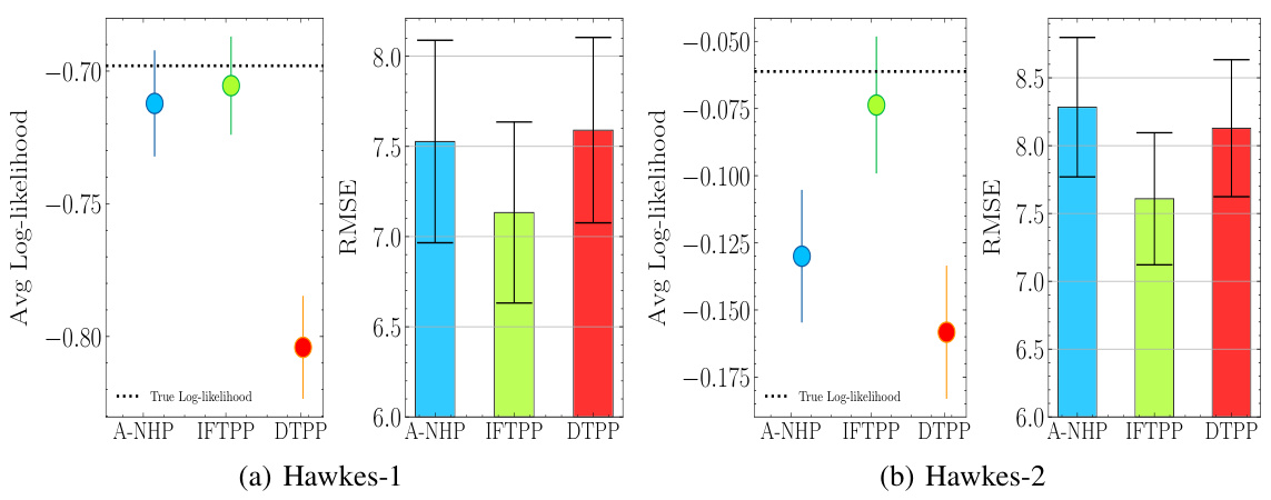
🔼 This figure compares the performance of the proposed Decomposable Transformer Point Process (DTPP) model and the Attentive Neural Hawkes Process (A-NHP) model on a synthetic dataset generated using a Self-Attentive Hawkes Process (SAHP). The left panel shows the average log-likelihood for each model, with error bars representing the 95% confidence intervals. The right panel shows the Root Mean Squared Error (RMSE) for each model, again with error bars representing the 95% confidence intervals. The figure demonstrates that DTPP achieves a comparable log-likelihood while showing lower RMSE, indicating better performance.
read the caption
Figure 2: Performance comparison between DTPP and A-NHP over the SAHP-Synthetic dataset.

🔼 This figure displays the goodness-of-fit results for five real-world datasets using the proposed DTPP model and five other strong baseline models. The goodness-of-fit is measured using average log-likelihood. The results demonstrate that the DTPP model outperforms the baselines across all datasets. The error bars represent 95% bootstrap confidence intervals.
read the caption
Figure 1: Goodness-of-fit evaluation over the five real-world datasets. We compare our DTPP model against five strong baselines. Results (larger is better) are accompanied by 95% bootstrap confidence intervals.
🔼 This figure displays the goodness-of-fit results for five different real-world datasets, comparing the proposed DTPP model against five other strong baseline models. The goodness-of-fit is measured using average log-likelihood. Error bars representing 95% bootstrap confidence intervals are included to show the uncertainty in the estimations. The figure shows that the DTPP model generally outperforms the baselines across the five datasets.
read the caption
Figure 1: Goodness-of-fit evaluation over the five real-world datasets. We compare our DTPP model against five strong baselines. Results (larger is better) are accompanied by 95% bootstrap confidence intervals.
More on tables

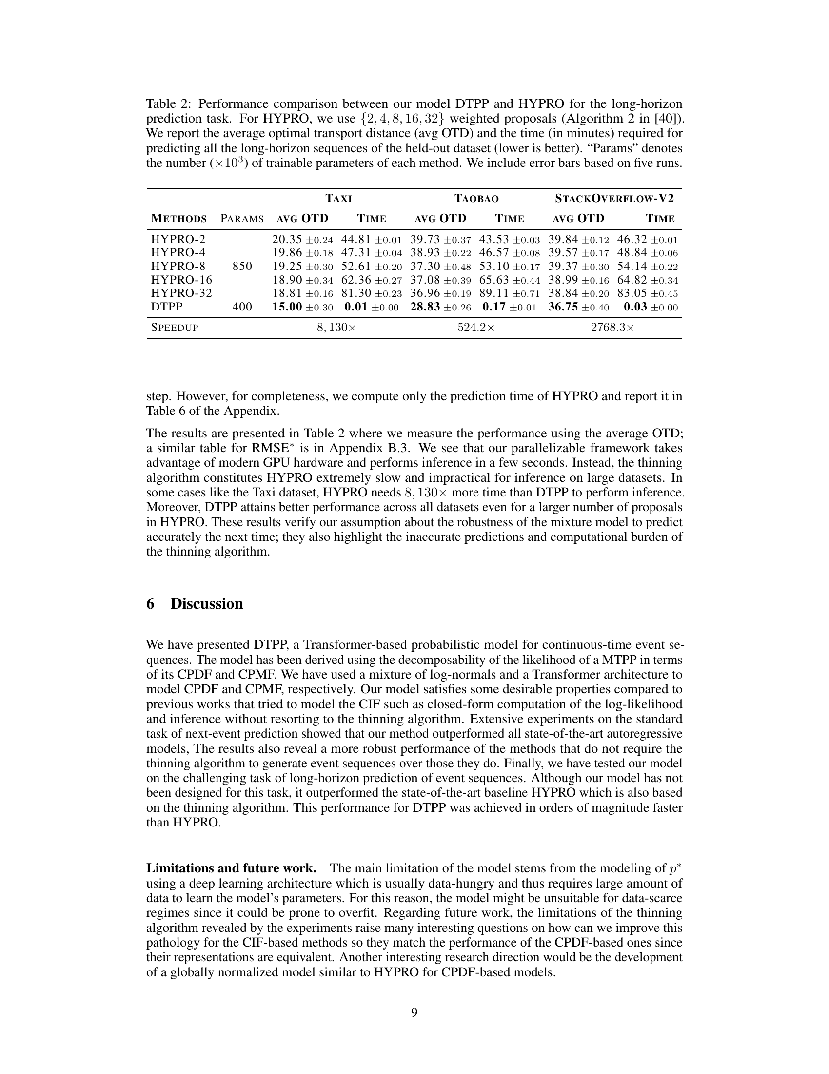
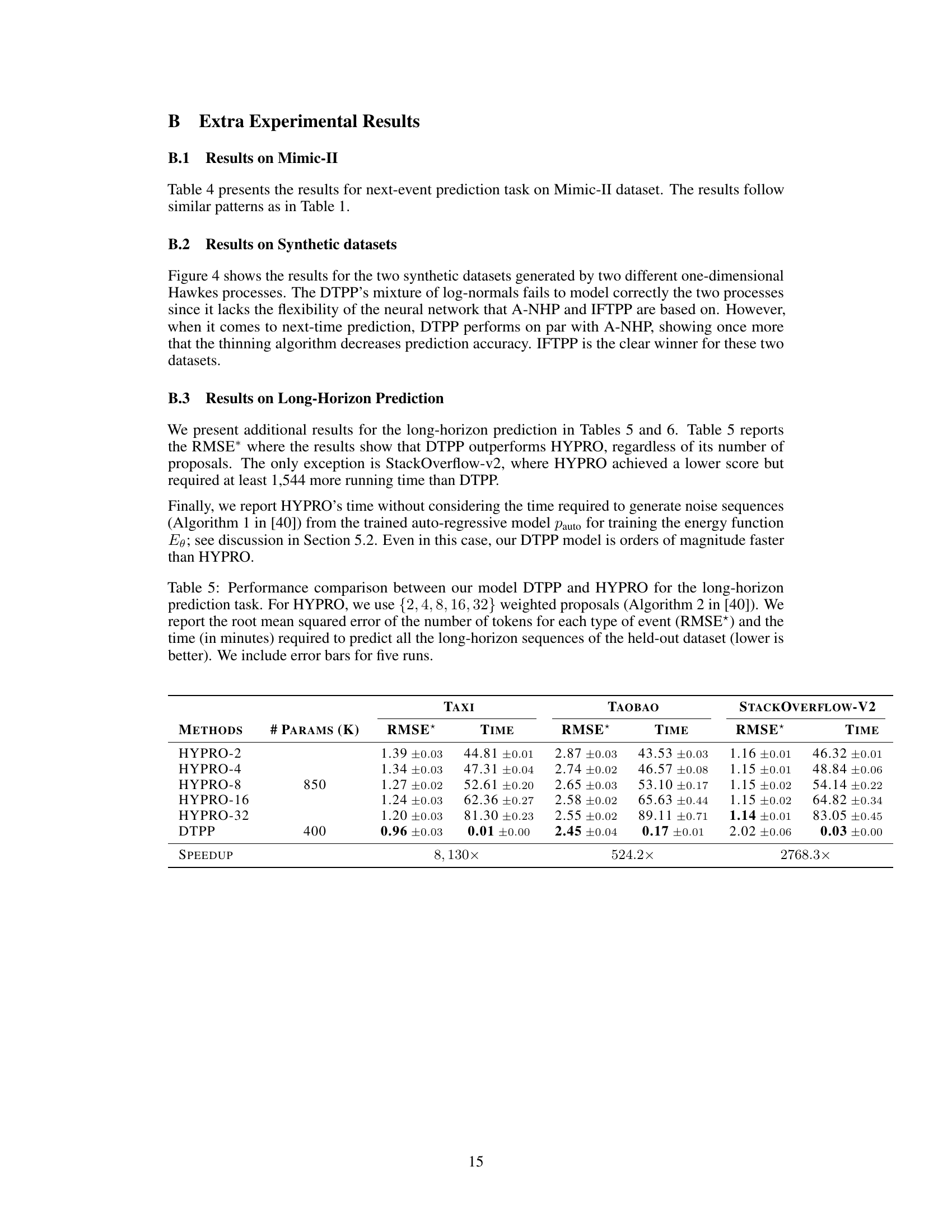
🔼 This table compares the performance of the proposed model (DTPP) and HYPRO on the long-horizon prediction task. It shows the average optimal transport distance (OTD) and the time taken to predict all sequences in the held-out dataset. HYPRO uses different numbers of weighted proposals (2, 4, 8, 16, and 32). Lower values for OTD and time are better. The table also provides the number of trainable parameters for each model and shows the speedup achieved by DTPP compared to HYPRO.
read the caption
Table 2: Performance comparison between our model DTPP and HYPRO for the long-horizon prediction task. For HYPRO, we use {2, 4, 8, 16, 32} weighted proposals (Algorithm 2 in [40]). We report the average optimal transport distance (avg OTD) and the time (in minutes) required for predicting all the long-horizon sequences of the held-out dataset (lower is better). “Params

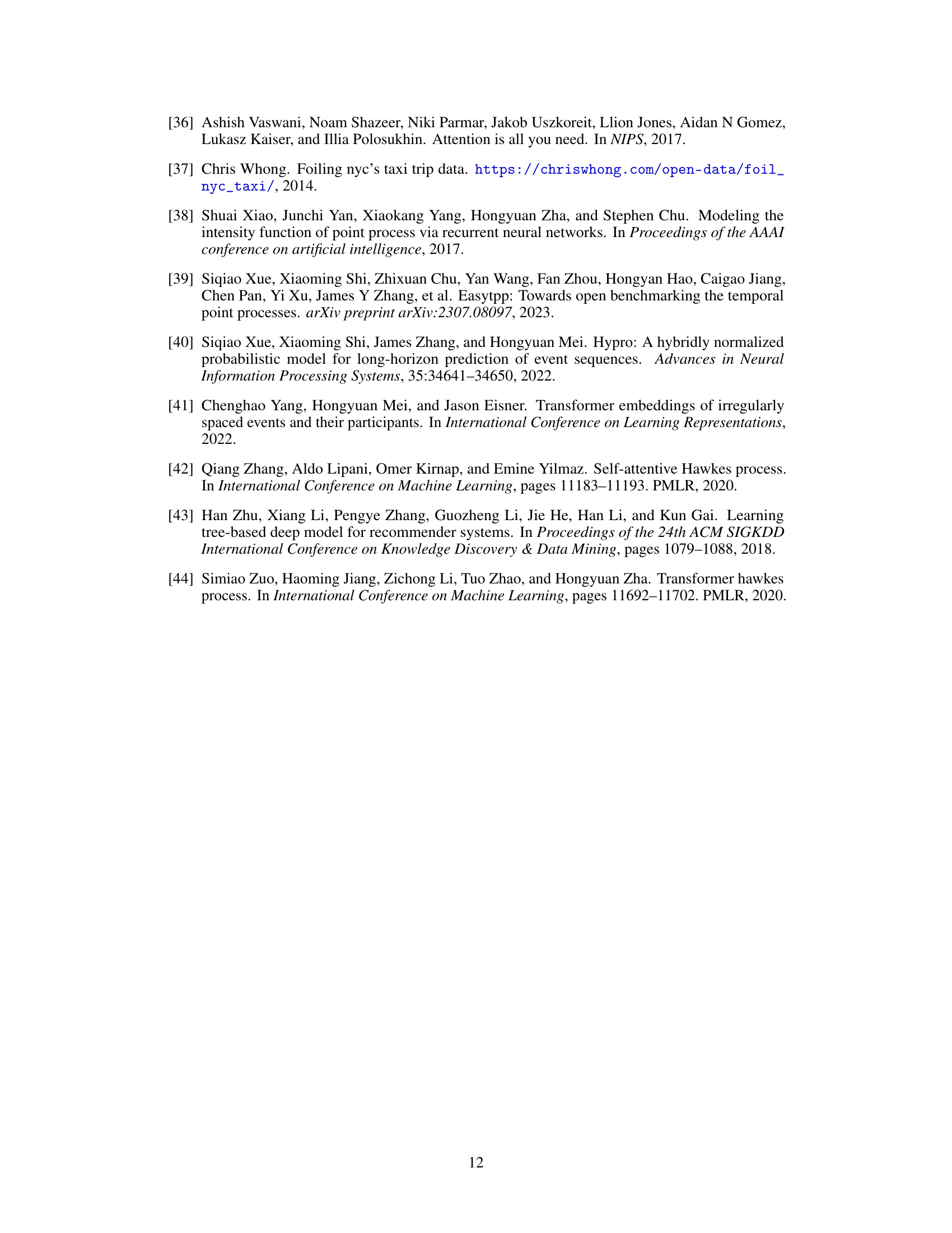
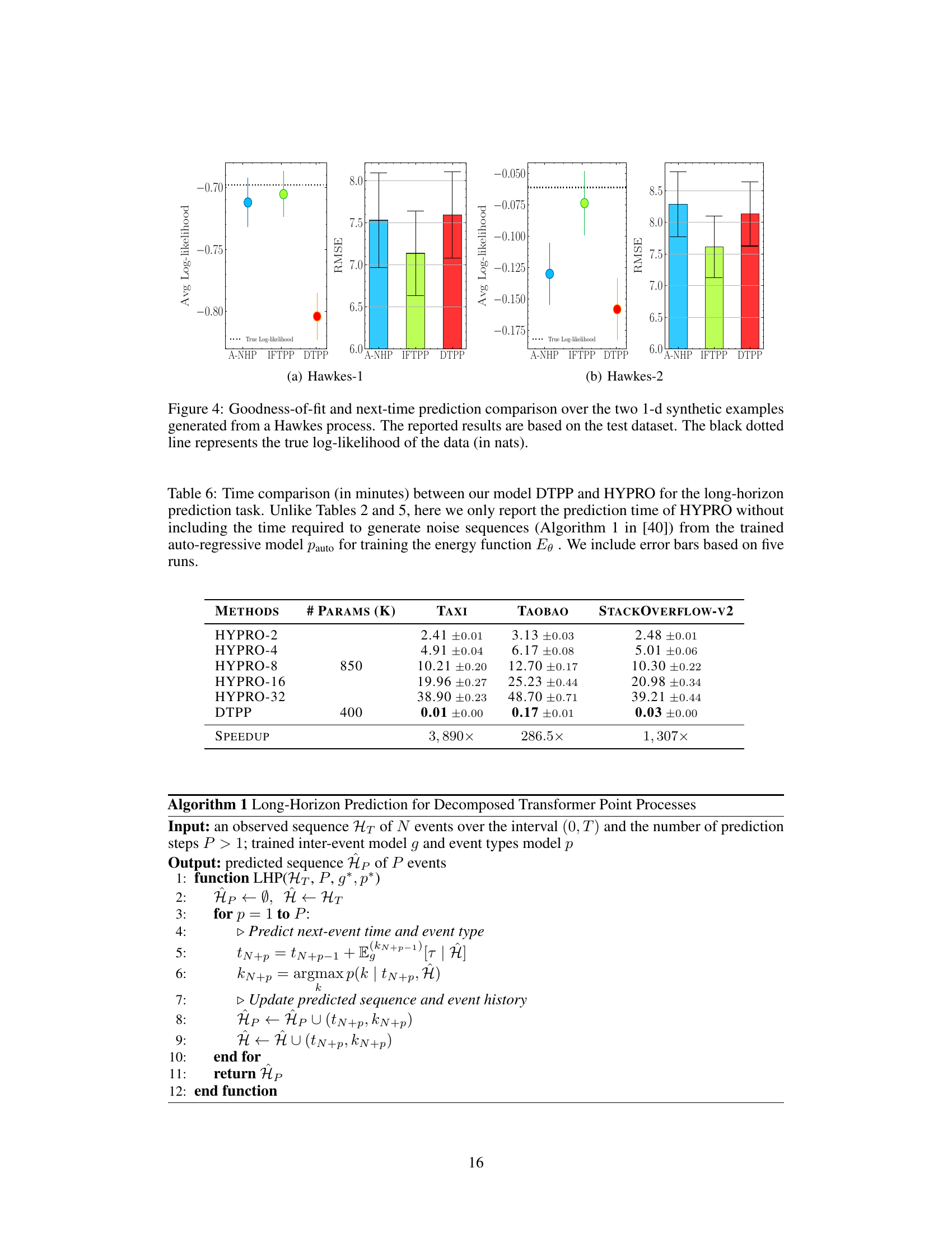
🔼 This table presents a summary of the characteristics of the datasets used in the paper’s experiments. For each dataset, it lists the number of event types (K), the number of event tokens in the training, validation, and development sets, and the minimum, mean, and maximum sequence lengths. The datasets include synthetic datasets generated from Hawkes processes and real-world datasets such as MIMIC-II, Amazon reviews, taxi trips, Taobao transactions, and Stack Overflow questions.
read the caption
Table 3: Characteristics of the synthetic and real-world datasets.
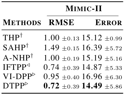
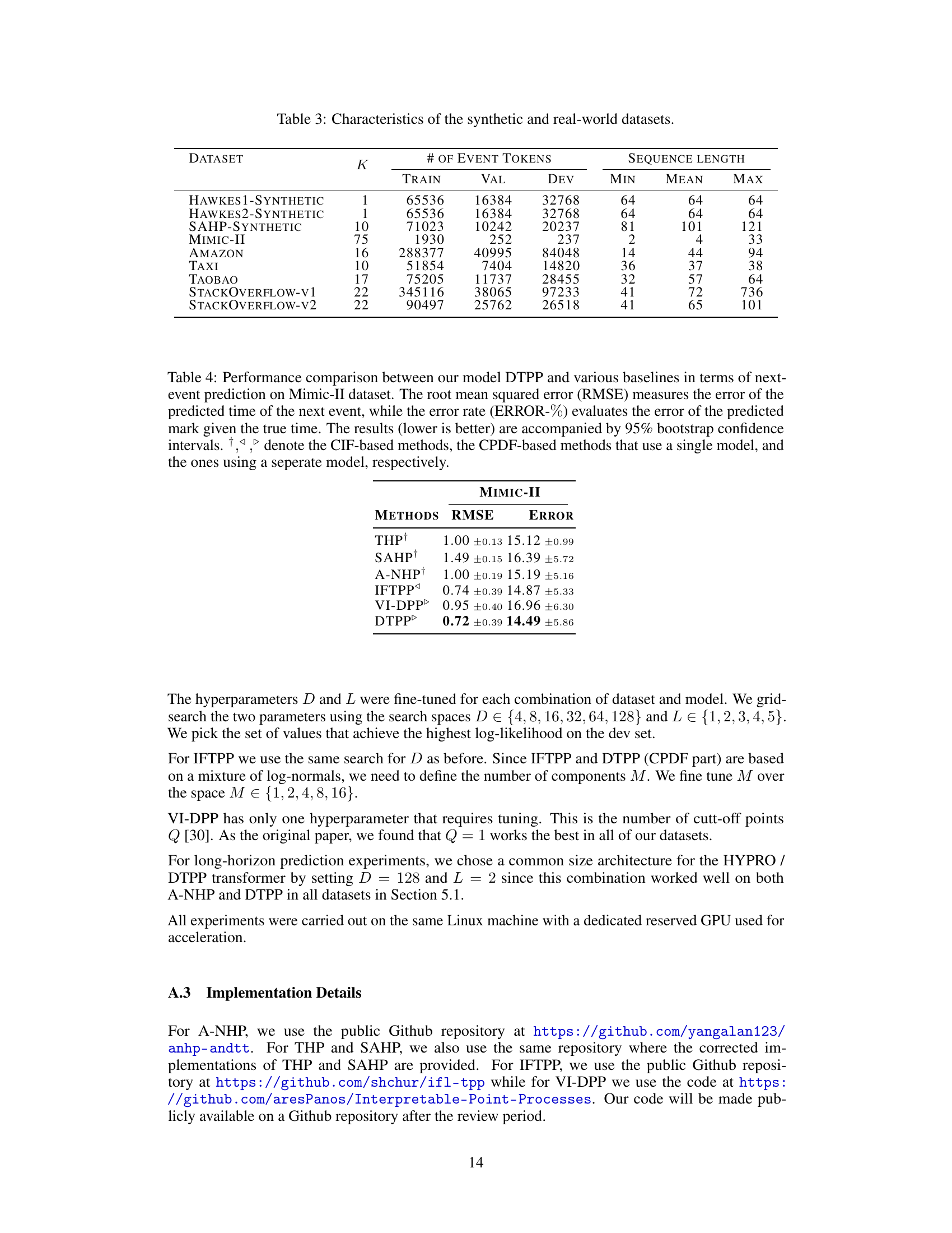
🔼 This table compares the performance of the proposed DTPP model and other baseline models on the MIMIC-II dataset for next-event prediction. It reports the root mean squared error (RMSE) for the predicted time and error rate for predicted event type. Lower values are better. The table also categorizes models as CIF-based (using conditional intensity function), single CPDF-based (using conditional probability density function with one model), and separate CPDF-based (using conditional probability density function with separate models for time and mark).
read the caption
Table 4: Performance comparison between our model DTPP and various baselines in terms of next-event prediction on Mimic-II dataset. The root mean squared error (RMSE) measures the error of the predicted time of the next event, while the error rate (ERROR-%) evaluates the error of the predicted mark given the true time. The results (lower is better) are accompanied by 95% bootstrap confidence intervals. †, ▷ denote the CIF-based methods, the CPDF-based methods that use a single model, and the ones using a seperate model, respectively.

🔼 This table compares the performance of the proposed DTPP model against HYPRO, a state-of-the-art long-horizon prediction model, across three real-world datasets (Taxi, Taobao, and StackOverflow-V2). The comparison is based on the average optimal transport distance (OTD), a metric for measuring the dissimilarity between event sequences, and the inference time required to generate the predictions. HYPRO uses a thinning algorithm, which is computationally expensive, while DTPP uses a more efficient approach. The number of trainable parameters for each model is also listed. The results demonstrate the superior efficiency and often superior accuracy of DTPP compared to HYPRO across all three datasets.
read the caption
Table 5: Performance comparison between our model DTPP and HYPRO for the long-horizon prediction task. For HYPRO, we use {2, 4, 8, 16, 32} weighted proposals (Algorithm 2 in [40]). We report the average optimal transport distance (avg OTD) and the time (in minutes) required for predicting all the long-horizon sequences of the held-out dataset (lower is better). “Params” denotes the number (×103) of trainable parameters of each method. We include error bars based on five runs.

🔼 This table compares the performance of the proposed DTPP model against the HYPRO model for long-horizon prediction. It shows the average optimal transport distance (OTD) and the computation time (in minutes) for both models across three datasets (Taxi, Taobao, StackOverflow-V2). HYPRO uses a varying number of weighted proposals (2, 4, 8, 16, 32), while DTPP uses a single model. The table highlights the significant speed advantage of DTPP over HYPRO, especially as the number of proposals increases.
read the caption
Table 2: Performance comparison between our model DTPP and HYPRO for the long-horizon prediction task. For HYPRO, we use {2, 4, 8, 16, 32} weighted proposals (Algorithm 2 in [40]). We report the average optimal transport distance (avg OTD) and the time (in minutes) required for predicting all the long-horizon sequences of the held-out dataset (lower is better). “Params
Full paper#
